Condensation
Organizing information across a family of observations. Define latent models, examine reconstruction and conditional independence, and prove an exact and quantitative correspondence theorem. A worked hierarchical-clustering example, and how condensation relates to earlier work in statistics and what remains between the theorem and useful translation between the latents of human and AI models.
By Satya Benson
1. Prerequisites
- Probability on finite sets, conditional probability, and elementary proofs.
- Conditional entropy and conditional independence; Section 1.1 collects what we use.
Condensation
- Construct latent models and check the three conditions on them: the latent variable model condition, reconstruction, and the Markov condition.
- Explain why a single agent would want its latents to satisfy the last two.
- Prove correspondence between families of latents, first exactly and then with explicit error terms.
A hierarchical clustering example
- Compare how different latent models of the same law meet the conditions, and what the conditioned score charges each for a query.
Condensation in context
- Relate condensation to natural latents, sufficient statistics, common information, computational mechanics, and graphical models.
- Separate informational correspondence from learning, finding, and using a translation.
- Identify which additional claims would connect correspondence to AI safety.
How to use this sheet
After the first lecture, read Sections 2.1 and 2.2 and work Exercises 2.1, 2.2 and 2.4. After the second lecture, read Sections 2.3 and 2.4 and work Exercises 2.5, 2.6, 2.7, 2.8, 2.9 and 2.10. These nine starred exercises, about 140 minutes in all, are the core route. Then read Sections 3 and 4, take the discussion prompts in Section 4.5 to your group, and finish with the quiz in Section 5. Exercises 2.3, 2.11, 2.12 and 3.1 are optional.
1.1 Information theory reference
All random variables have finite ranges and all logarithms are base two. For a finite-valued variable ,
with . Conditional entropy is nonnegative. It is zero precisely when is a function of almost surely: values on probability-zero events do not matter. The chain rule and conditioning inequality are
Conditional mutual information is
It is symmetric in and is zero precisely when are conditionally independent given . Omitting gives mutual information . Entropy of a tuple means joint entropy, not the sum of its marginal entropies. An empty tuple is constant and has zero entropy. For probability distributions on a finite set,
This last quantity appears only in the optional score discussion.
2. Condensation
In empirical work, people look for features in AI systems which correspond robustly to human concepts. In general, these can be hard to find.
One ambitious approach to this problem is to think through from first principles how agents in general might organize information about the world into concepts.
How should information be broken into reusable pieces? Is there one way to do this which many different kinds of agents will converge on?
We will propose two conditions that we think are normative for agents in general: conditions an agent will want its own organization of information to satisfy. Under those conditions, corresponding families of latents in two models determine one another.
2.1 A family of questions
Fix jointly distributed observables . We look for latent variables, each assigned to a set of observations, such that the latents assigned to an observation determine it. We will give conditions under which corresponding families of latents in two such models determine one another, and bound the remaining conditional entropy when the conditions hold approximately. We take the joint distributions as given.
Remark (Choosing the observables). One can think of each as a function of a single underlying variable representing sense data or a physical state. This introduces no restriction: that variable could simply be the tuple of all observations. An observable distinguishes outcomes by partitioning them into its possible answers; random-variable values label those parts. Information quantities do not depend on bijective relabeling of answers. The choice of which observables to include, and their joint law, remains part of the model.
Example 2.1 (Overlapping observations). Let be independent fair bits and set
Use a latent for observations 1 and 2, a latent for observations 1 and 3, and a latent for observations 2 and 3. Each observation is determined by the two latents assigned to it. Each of these latents can also be recovered from either observation to which it is assigned.
2.1.1 Addresses and families
Let and write for its nonempty subsets. An address specifies which observations receive a latent . We use one latent for each nonempty subset, setting unused ones to constants, and order the addresses by inclusion.
Definition 2.2 (Latent model). A latent model of consists of finite-valued variables jointly distributed with , such that
Here for a family .
We call (1) the latent variable model condition, or LVM. The contributing latents, taken together, determine the observation; some of them may represent residual noise.
For nonempty and , define two different families:
The tuple is the tower above . The tuple contains all latents contributing to at least one observation in ; we call these latents active for . They determine . In particular is the family of addresses contributing to , so (1) reads . For a larger , and generally differ.
Glossary. The sheet uses a small fixed vocabulary.
Address A nonempty . The model has one latent at each address; unused ones are constant.
Block A nonempty set of observations, with .
Family A set of addresses, and the corresponding family of latents .
Contributing contributes to when . The contributing family of is .
Tower The family of latents at and every address containing it.
Active is active for a block when , that is, when it contributes to some observation in . The active family is .
Upward closed A family containing every superset of each of its addresses (Section 2.2).
Witness A variable from which a target is recoverable (Section 2.3).
Exercise 2.1 (★) (Overlapping bits; 15 minutes). Use Example 2.1, with all unmentioned latents constant.
(a) Compute , , and .
(b) List , , and , including constant latents. Which tuple determines ? Which of the three is ?
(c) Give explicit functions recovering from its contributing latents and recovering from .
(d) Does the address structure have to be a tree? Identify two overlapping addresses in this example neither of which contains the other.
Solution
The independent fair bits are , and , , .
(a) . The tuple of all observations determines and is determined by it, so . The pair already determines all three bits, hence
Its shared bit is .
(b) The families, including constant latents, are
The first tuple has nonconstant entries , so determines . Intersecting the first two families leaves , the third family listed, whose only nonconstant content is .
(c) Recover by taking the ordered pair . Recover from by projecting onto its first coordinate.
(d) Addresses and overlap but neither contains the other. Thus the contribution pattern need not form a nested tree.
2.2 Two conditions on a latent model
Every observable law has trivial latent models: put a copy of each in its singleton latent, or the entire tuple in the top latent , and LVM holds either way. So LVM alone says nothing about how information is shared. Two further conditions do.
Definition 2.3 (Reconstruction). A latent model has exact reconstruction if
Equivalently, whenever : every latent in that finite tuple can be recovered from .
The equivalence in this definition uses exact zero errors. In approximate statements we will bound the entropy of the whole tower; separately small errors for its individual latents could add up.
A family is upward closed if and imply . For example, and are upward closed. Upward closure makes a family include every more general latent that its members may depend on.
Definition 2.4 (Markov condition and defect). The Markov condition is
for all upward-closed families . Its quantitative defect is
The condition says that the latents at the shared addresses account for the dependence between the two families. In the two-observable case, its only potentially nonzero requirement is
This is a graphical-model condition for the inclusion order. The equivalent local version says that each latent is conditionally independent of all incomparable latents given its strict supersets.
Definition 2.5 (Perfect condensation). A latent model is a perfect condensation if it has exact reconstruction and satisfies the Markov condition.
This is equivalent to Eisenstat's definition by optimal conditioned scores (Eisenstat 2025, Theorem 5.10). Section 2.6 explains that connection. The overlapping-bit model in Example 2.1 is a perfect condensation. All nonconstant latents are mutually independent, so disjoint subfamilies are independent, including after conditioning on the remaining common subfamily. Reconstruction follows from coordinate projections.
Exercise 2.2 (★) (Two failed models; 20 minutes). Keep the observables of Example 2.1. Consider two alternative models.
(a) Set for and every other latent constant. Check LVM and reconstruction. Take and . Calculate the conditional mutual information in Definition 2.4. Which information is duplicated across singleton latents?
(b) Instead set and every other latent constant. Check LVM and the Markov condition. Compute . Which condition fails?
(c) Explain why LVM, reconstruction, and the Markov condition have different roles.
Solution
(a) In the singleton-copy model , the contributing family for includes itself. Thus LVM holds. Each nonconstant latent has just one contributing observation, from which it is recovered identically, so reconstruction holds too.
For and , all entries of are constant. The only nonconstant entries of the two larger tuples are and . Consequently
Both singleton latents determine , while their common ancestor latents are constant. This violates the Markov condition. It is enough to exhibit this one pair of upward-closed families; finding the maximum defect is unnecessary.
(b) With only nonconstant, each observation is obtained by projection, so LVM holds. Every nonempty upward-closed family contains the top address. If both families are nonempty, their intersection contains that top latent and determines all latent variables; the conditional mutual information is zero. If either is empty it is zero as well. Thus the Markov condition holds.
But leaves the independent fair bit unknown, so
Reconstruction fails.
(c) LVM requires enough latent information to determine each observation. Reconstruction excludes information placed at a shared address that an individual contributing observation cannot recover. The Markov condition excludes dependence between families not accounted for by their common latents. The singleton model satisfies reconstruction but fails the Markov condition; the top-latent model satisfies the Markov condition but fails reconstruction.
2.2.1 Existence is a separate question
The preceding examples test particular latent models. A stronger question is whether a given observable law admits any perfect condensation. Even a pair of correlated binary variables can fail to do so.
Let , let be a fair bit, and set , where is independent Bernoulli noise and . Here is addition modulo two, so is when the two bits agree and when they differ. The joint law is
All four outcomes have positive probability, and are dependent because the two rows differ (). Suppose a perfect condensation existed, and consider its top latent .
With two observations there are only three addresses, so the whole model is three latents:
LVM says is determined by and by . The top latent is the only one assigned to both observations, so it is the only place shared information can sit.
Reconstruction would give almost surely. Because all four observable pairs have positive probability, these equalities force
Thus is constant. The Markov condition would then require and to be independent. LVM makes each a function of its singleton latent and the constant . Functions of independent variables are independent, contradicting the chosen observable law. No perfect condensation exists for this pair.
There is a quantitative obstruction if we retain exact reconstruction. The same argument makes constant. Data processing then gives
where is the binary entropy function. Dependence between the observables must remain as a Markov defect when their separately recoverable top latent is constant. The bound is attained by the singleton-copy model , with constant top.
That bound pins one end of a trade-off: exact reconstruction forces a Markov defect of at least , and tolerating some reconstruction error buys part of it back. When no perfect condensation exists, which is the usual situation (Exercise 2.3), the latent models of a given observable law trace out a Pareto frontier between reconstruction defect and Markov defect. The useful question is then whether some point on that frontier has both low enough for the correspondence bound of Section 2.3 to say something.
Exercise 2.3 (Full support; optional, 10 minutes). The argument for the noisy pair used only two facts: every combination of values has positive probability, and the observables are dependent. Generalize it. Suppose every combination of values that can individually take has positive probability.
(a) Show that in any perfect condensation, every latent at an address with at least two elements is constant.
(b) For disjoint nonempty blocks , apply the Markov condition to and to show that and are independent. Conclude that a perfect condensation exists exactly when the observables are mutually independent.
Solution
(a) Let contain . Reconstruction gives almost surely. Every pair of values has positive probability, so for all of them, and and are the same constant.
(b) Every address in meets both disjoint blocks, so it has at least two elements and its latent is constant. The Markov condition therefore makes and independent, and by LVM and are functions of them. Taking and for factorizes the joint law into its marginals. Conversely, if the observables are mutually independent, the singleton-copy model is a perfect condensation: LVM and reconstruction are immediate, and the Markov condition holds because all its nonconstant latents are mutually independent, as for the overlapping-bit model.
In particular, a perfect condensation of any full-support law with dependent observables is impossible, which is why the approximate theorem is the one that applies to noisy data.
Exercise 2.4 (★) (Families, not individual latents; 15 minutes). For this exercise let , take independent fair bits , and set , . Compare
(a) Check that both models are perfect condensations.
(b) Compute .
(c) Show that and determine one another. Explain why correspondence between these tuples is a different claim from correspondence between the singleton latents.
Solution
Here are independent fair bits. In model the three latents are ; in model they are .
(a) Both contributing families determine their observations. All latents are recoverable from each observation to which they contribute. For example, is the first coordinate of either or , and . For two observables the only nontrivial Markov requirement is independence of the two singleton latents given the top latent. For this is . For it is
Both are therefore perfect condensations.
(b) .
(c) The tower at consists of , and the tower consists of . Each is a deterministic function of the other. A copy of the higher-address information can appear in a lower latent without changing the tower's total information. Thus the individual latents need not correspond even when the relevant towers do.
2.2.2 Why we ask for the conditions only approximately
Figure 1 shows a hierarchical model of 36 labelled points, worked through in Section 3. A global shape is assigned to every point, a group center to the 18 points of its group, and a cluster center to the nine points of its cluster.
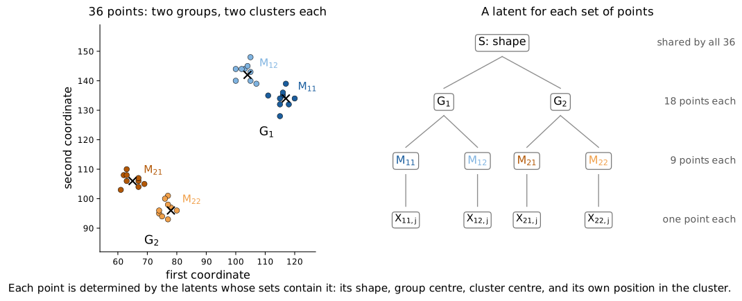
One draw from the finite model. The left panel shows the 36 points; the right panel shows which set of observations receives each parameter. The global shape is available to every observation.
The cluster center specifies a distribution for its points, not the points themselves, so a point does not determine the center it was drawn from:
Every kernel here has full support: no finite set of points pins a parameter. LVM and the Markov condition hold exactly here. The reconstruction condition holds only approximately. So we ask for reconstruction up to a defect: for ,
and prove a correspondence whose error grows with and .
2.3 The correspondence theorem
Take two latent models of the same observable tuple . To compare them, put on one probability space while retaining both specified laws and . For finite variables this is always possible: for example, use . The theorem holds for any such coupling.
Theorem 2.6 (Correspondence). For two latent models of and any nonempty , let . Then
If each term in the sum is at most and , the bound is . If both budgets are , it is . Interchanging gives the reverse bound.
Corollary 2.7 (Exact correspondence). If and are perfect condensations, their towers above every nonempty address determine one another almost surely:
The forward bound uses reconstruction in , LVM in , and the Markov defect of . It does not use the Markov condition of until we reverse the argument. The result concerns corresponding families. Exercise 2.4 shows why we cannot simply replace those families by individual latents.
This proof is a specialization of Eisenstat's approximate correspondence theorem (Eisenstat 2025, Theorem 6.8), using the two-witness inequality (Eisenstat 2025, Lemma 6.4). The exercises below give the full argument without additional machinery.
2.3.1 Proof roadmap
The theorem has three steps.
- If two witnesses each determine a target and are independent given their common part, that common part determines the target. Entropy gives a version with errors.
- Each observation is determined by its contributing -latents. Anything recoverable from is therefore recoverable from that family.
- Intersect these contributing families over . Exactly the addresses containing all of survive. Each intersection costs at most one Markov error term.
The word "witness" below means a variable or tuple from which the target is recoverable.
Lemma 2.8 (Two witnesses). For any finite-valued variables ,
Exercise 2.5 (★) (Prove the two-witness lemma; 20 minutes). (a) Prove Lemma 2.8 by expanding conditional entropies using the chain rule. Find an expression for the difference between the right and left sides that is a sum of nonnegative quantities.
(b) Deduce the exact statement when the three terms on the right are zero.
(c) Explain the three error terms. Which measure failures of reconstruction, and which measures dependence that remains after revealing ?
Hint
Try expanding , then rearranging with the chain rule, which is stated in Section 1.1. The desired difference contains a conditional mutual information and a conditional entropy.
Solution
For arbitrary finite , expand the two conditional mutual informations in entropies and regroup the terms in pairs:
Rearranging gives
Its right side is nonnegative, which proves the lemma.
If , the inequality and nonnegativity imply . Thus a target recoverable from each witness is recoverable from their designated common part when the witnesses are conditionally independent given that part.
The first two terms measure what each witness, together with , still fails to determine about . The third measures dependence between not accounted for by . No independence assumption is needed for the inequality itself; exact independence is the case where the third error is zero.
Exercise 2.6 (★) (The dependence term is needed; 5 minutes). Let be a fair bit and let be constant. Evaluate every term in (3). What would go wrong if the mutual-information term were omitted? How does this example resemble the singleton-copy model in Exercise 2.2?
Solution
With a fair bit and constant,
The inequality is the equality . Without its mutual-information term it would assert . The two witnesses each determine the same bit while the designated common variable is constant, as in the singleton-copy model of Exercise 2.2.
Exercise 2.7 (★) (Transfer through an observable; 10 minutes). Let be any finite-valued target and suppose is determined by . Prove
State the equality obtained by adding to the conditioning tuple, then apply the conditioning inequality. Does this argument assume that and are conditionally independent given ?
Solution
If is a function of almost surely, adding to that conditioning tuple changes no information. Hence
The inequality is conditioning monotonicity. It does not assume that and are conditionally independent given . They can share additional information beyond .
Exercise 2.8 (★) (Intersect the address families; 15 minutes). (a) For , list , , and . Compute and then its intersection with .
(b) Show that an intersection of upward-closed families is upward closed.
(c) For general nonempty , prove by checking membership of an address on both sides.
(d) If are upward closed, apply the two-witness lemma with , , and . Why can the extra conditioning on be dropped from each reconstruction term? Write the resulting bound using .
Solution
(a) The first two families are listed in Exercise 2.1, and
Thus , and intersecting with leaves only .
(b) If belongs to every family in an intersection and , upward closure places in each such family, hence in the intersection.
(c) For an address ,
(d) Put , , . The tuple is a subtuple of both and . Thus and similarly for . By the definition of , the lemma gives
Upward closure is needed to invoke the bound .
Exercise 2.9 (★) (Complete the correspondence proof; 25 minutes). Fix and set . We prove, for ,
(a) Use Exercise 2.7 to prove (4) at .
(b) Use Exercise 2.8 to show, for ,
(c) Conclude (4) by induction. Evaluate it at to prove Theorem 2.6, and check the case explicitly.
(d) Deduce Corollary 2.7, including the reverse direction. Name the assumption used at each step of the proof.
(e) Suppose instead that separately for all relevant addresses . Why does this not by itself supply the tower error budget ?
Solution
Fix a nonempty , put . Every is upward closed, as is every by Exercise 2.8. We prove (4) for .
For , , and Exercise 2.7 gives . This is the claimed bound with zero intersection terms.
Suppose (4) holds for , where . Apply Exercise 2.8 to the upward-closed families and . Their intersection is , so
The second line uses the induction hypothesis and Exercise 2.7. This completes the induction. At , Exercise 2.8 gives , hence
For this is exactly the observable-transfer inequality, so no intersection or Markov error is required. There are reconstruction errors and Markov defects. Bounding each reconstruction error by and each Markov defect by gives , or for a common budget.
If are perfect condensations, each reconstruction error is zero: for every and , reconstruction says is a function of . The finite tuple of such variables is consequently a function of . Also . The inequality gives zero conditional entropy in the forward direction. Interchanging , using reconstruction in and , proves the reverse direction. Zero conditional entropy is almost-sure deterministic recoverability in our finite setting.
The proof uses LVM in for Exercise 2.7, reconstruction in to bound those errors, and the Markov condition of at intersections.
Finally, approximate errors for individual latents do not directly give the same error for a tuple. For example, if two independent fair bits remain unknown given a constant observation, each conditional entropy is one bit but the tuple's is two bits. Conditional subadditivity gives a sum of the individual budgets, not a single budget. The theorem states its hypothesis in terms of tower errors to avoid this ambiguity.
2.4 Why an agent would want these conditions
The correspondence theorem is meant to show when the latents of different agents correspond, so the conditions should not be motivated by correspondence itself. They should serve a single agent's own interests. This section gives two such readings.
The conditioned score. Suppose an agent stores each latent given the more general ones, and answers a query about an observation block by reading every latent active for , most general first. Its expected description length is the conditioned score
Every strict superset of an address meeting also meets , so the conditioning is available when reading in reverse inclusion order. Put . Then
The second term charges latent information not recoverable from . The first charges dependence not accounted for by the inclusion hierarchy. It vanishes under the Markov condition. Exercise 2.12 proves the decomposition.
An agent that answers queries about a block pays , and no latent model does better than . The gap splits into exactly our two defects. Short descriptions for the queries an agent cares about are small defects. For , the singleton gap bounds , the reconstruction hypothesis of Theorem 2.6 (Exercise 2.12). So the conditions need not be assumed as a coincidence: efficient agents buy them. Efficiency is relative to the blocks an agent actually queries, and there is not always a single model minimizing the score for every block.
Reconstruction: no dead weight. The concept at is used whenever any observation in is. Information that only some of those circumstances can use is stored where it is dead weight most of the time the concept is used. The reconstruction error measures exactly the part of the concept that a query about pays for but cannot pin down. In the top-latent model of Exercise 2.2, carries the bit , which is dead weight whenever the concept is used for .
Markov: local inference. The Markov term also has a reading that does not mention description length. Once the more general concepts are known, a concept should bear only on the observations in its own scope:
Then when the agent learns or revises something about the concept at , it never has to revise its beliefs about observations outside , except through 's more general context. Given LVM and reconstruction, (6) holds for every address exactly when the Markov condition does.
Exercise 2.10 (★) (Local inference; 15 minutes). (a) In the singleton-copy model of Exercise 2.2, compute the left side of (6) for .
(b) Let , let be a fair bit, and set . File at every pair address, , with every other latent constant. Check LVM and reconstruction. Compute the left side of (6) for , and find upward-closed families violating the Markov condition. Where should be filed instead?
(c) Prove that the Markov condition implies (6). Apply Definition 2.4 to and , and identify their intersection.
(d) Assume reconstruction. Show that and determine one another. Conclude that (6) for every is the local version of the Markov condition stated after Definition 2.4.
Solution
(a) Here and every strict superset of holds a constant, so the left side is . The pair determines , hence , so this is . The concept at carries two bits about observations outside its scope that no more general concept accounts for.
(b) Each observation equals a latent assigned to it, for example , so LVM holds. Every nonconstant latent equals for each in its address, so reconstruction holds. The only strict superset of is , whose latent is constant, so the left side is . For and the intersection is , and . The bit is shared by all three observations, so it belongs at the top address: with every other latent constant is a perfect condensation.
(c) An address meets exactly when . So consists of the addresses that contain but are not contained in it: the strict supersets of . Both families are upward closed, so the Markov condition gives
The tuple is part of , and by LVM is a function of , which contains for every . Conditional mutual information cannot increase when either side is replaced by a function of it, so the left side of (6) is zero.
(d) Every contains some , and reconstruction makes a function of . So is a function of , and the previous part gave the converse. The left side of (6) therefore equals . The family consists of the strict supersets of , on which we condition, and the addresses incomparable with . So the quantity vanishes exactly when is conditionally independent of the incomparable latents given its strict supersets. Required for every , this is the local version of the Markov condition, which is equivalent to it.
2.5 Optional: several observations as one witness
A shared parameter need not be recoverable from a single observation. For example, take , let be a fair bit, and set , where the are independent Bernoulli noises with , independent of . The model , satisfies LVM and the Markov condition exactly, but , where is the binary entropy function of Section 2.2.1. Larger observation blocks can reveal more about . To use them in the proof, replace by .
Exercise 2.11 (Block witnesses; optional, 25 minutes). (a) Let and suppose a target has conditional entropy at most given each of , , and . Which addresses survive the intersection ? Prove a bound on the entropy of given the surviving -latents.
(b) More generally, let be a nonempty finite family of nonempty observation blocks. Adapt Exercise 2.9 to show
(c) Fix an integer and take every -element subset of as a witness. Show that exactly when . What does this give for ? Why is generally larger for ?
Solution
(a) A nonempty address meets each of precisely when . A singleton misses the complementary pair; every address with at least two elements meets every pair. Thus the surviving tuple consists of the three pair latents and the top latent. Applying the two-witness lemma twice, after observable transfer for each block, gives
It does not isolate the top latent alone.
(b) For each block , the family determines : for every it contains . Exercise 2.7 therefore extends to . Each is upward closed. Enumerate and intersect the first contributing families. Exactly the induction in Exercise 2.9, now with these families as leaves, gives
For this is just the transfer inequality. We required a nonempty family so the induction and the intersection count apply.
(c) An address fails to meet some -subset of exactly when contains at least elements. Thus it meets every such subset exactly when . For this says , recovering the tower. For an address can survive even if it misses some elements of ; is a larger family. If every witness error is at most , write to obtain the explicit bound . The restriction ensures witnesses exist.
Eisenstat's almost-perfect condensation (Eisenstat 2025) builds in block witnesses of this kind, with a threshold on that lets small latents absorb local noise.
2.6 Optional: more on the conditioned score
Compare the conditioned score of Section 2.4 with the simple score
which charges each latent active for separately, ignoring what the more general latents already say. Both are ideal expected description-length quantities.
For a graphical-model expression, define
This is a normalized distribution: sample larger addresses before smaller ones. Conditional kernels on probability-zero parent configurations can be chosen arbitrarily. Direct expansion gives . Thus (5) separates two nonnegative defects.
Exercise 2.12 (The two charges; optional, 25 minutes). (a) Order so strict supersets appear first. Use the chain rule and conditioning inequality to prove .
(b) Use LVM to prove , hence (5).
(c) For both models in Exercise 2.4, calculate and . Why is copying the top variable into a lower latent free under one score but not the other?
(d) If , show that .
(e) Prove that a latent model is a perfect condensation exactly when for every nonempty block , which is Eisenstat's definition.
Solution
(a) List as with strict supersets appearing before subsets. Such an order exists because strict inclusion has no cycles. Every strict superset of an active address also meets , so is in this list. Therefore
Summing and applying the chain rule gives , hence .
(b) Since determines , the joint entropy can be expanded in two ways:
Subtracting and adding proves
(c) In Exercise 2.4, the independent model has simple score and conditioned score . In model , the simple score is , while the conditioned score is
Both models determine , whose joint entropy is three. The conditioned score charges only the extra information below ; its copies add zero conditional entropy. The simple score charges those copies again.
(d) If , every meets . Thus is a subtuple of and
where the last inequality uses the nonnegative score decomposition.
(e) Let . For upward-closed , partition into
Order these blocks , internally by reverse inclusion. Upward closure ensures this order is valid and no latent in has a strict superset in , or conversely. Conditioning inequalities and chain rules within each block imply
The latter mutual information equals . Hence .
If all score gaps vanish, the decomposition forces , giving the Markov condition. The singleton gap at forces the contributing tuple, and therefore each latent at an address containing , to be determined by . This gives reconstruction.
Conversely, suppose reconstruction and the Markov condition hold. For every , each active latent is determined by some with , and hence by . Therefore . In a reverse-inclusion order, the earlier latents consist of all strict supersets of the current latent and some incomparable latents. The global Markov condition implies that conditioning on these extra earlier latents does not reduce its entropy beyond conditioning on strict supersets: apply the condition to the upward cone of the current address and the upward-closed family of earlier addresses. Their intersection is the strict-superset family. Thus the score's chain-rule inequality is an equality, . The decomposition gives for all .
Small score gaps therefore force small defects. The converse for Eisenstat's positive-threshold version needs extra reconstruction coverage (Benson 2026).
3. A hierarchical clustering example
3.1 Thirty-six observations
There are two groups, each containing two clusters, each with nine observations. Write for the th two-dimensional point in cluster of group . The labels and memberships are fixed. We are comparing models of this labeled family, not inferring an unknown partition of an unlabeled cloud.
The parameters are a global shape , group centers , and cluster centers . Given these parameters, the 36 observations are independent. Marginalizing over shared parameters generally makes observations dependent. The plotted cloud in Figure 1 is one realization; the random variables and their entropies refer to the joint law across realizations.
3.2 An explicit finite law
Let . Draw uniformly from three shape labels, and draw independently and uniformly from , independently of . Conditional on , draw its two centers independently:
Given and all centers, draw the observations independently, using
where
Each proportionality means normalization by the sum over . These are probability mass functions on a finite grid. The matrices control shape; they are not the exact covariances after discretization and boundary truncation. Every grid point has positive probability. Cluster centers tend to lie near their group center, but the four components need not be visually separated in every realization.
3.3 A structured latent model
Let contain all 36 indices. Let be the 18 indices of group , and the nine indices of cluster . Assign
and make every other latent constant. The joint law factorizes in the address inclusion order, so its Markov defect is zero.
LVM holds exactly because the singleton latent supplies the sampled point itself. The cluster center and shape alone only specify a distribution for the point, leaving residual conditional entropy .
Reconstruction is different. All the kernels have full support, so any finite observation block leaves several parameter configurations with positive posterior probability. For example, . The model's joint law satisfies the Markov condition exactly, but it is not a perfect condensation. Since every combination of points has positive probability and the points are dependent, no latent model of this law is (Exercise 2.3).
For a nonempty block , the general score-gap identity (5) is
Here the bracketed Markov term is zero. The gap is the latent information remaining uncertain after observing the queried block.
3.4 Three organizations of the same observable law
For a nonempty queried observation block , the conditioned score sums the charges of all latents active for .
One global tuple. Put and make every other latent constant. The global latent determines each observation. This is the top-latent model of Exercise 2.2 at scale: it satisfies the Markov condition but fails reconstruction. For every nonempty ,
This attains the entropy bound when querying the whole tuple. Even a singleton query incurs the entire tuple's entropy in this score.
An ordered chain. Choose an ordering . Set and make other latents constant. The contributing latents for contain . The charge for the latent holding is , hence
This attains the entropy bound for prefix queries. Querying only costs .
The structured model. The score charges the shape once, the group and cluster parameters needed by , and the residual uncertainty of each requested observation:
This expression avoids charging for unrelated observations. It need not be smaller than the other scores for every block. In particular, for it exceeds by the remaining parameter uncertainty, whereas both baseline constructions attain . Fitting the observable law does not by itself settle which organization is preferable across queries.
Exercise 3.1 (The three organizations and the conditions; optional, 10 minutes). (a) Show that the global and chain models satisfy the Markov condition. Why is it automatic for the chain?
(b) For a single point , describe the reconstruction error in each of the three models. How does it depend on in the chain, and on the number of observations in each model?
(c) None of the three models is a perfect condensation. Which comes closest to satisfying the conditions with a small tolerance?
Solution
(a) In the global model every nonempty upward-closed family contains the top address, whose latent is the only nonconstant one, so every Markov term conditions on everything, as in Exercise 2.2. In the chain, the nonconstant addresses are nested, so an upward-closed family contains exactly those with up to some bound: its nonconstant latents are for some . Of two such families, one's nonconstant latents are then those of the intersection, and the Markov term vanishes.
(b) In the global model the tower above is , so the error is : the uncertainty about all other points, which grows with their number. In the chain the tower is , so the error is : zero for the first point and growing along the ordering. In the structured model the tower is , so the error is : the parameter uncertainty a single point leaves, which does not grow with the number of observations.
(c) The structured model. It satisfies the Markov condition exactly, and its reconstruction errors are bounded by the parameter uncertainty one point leaves, uniformly in and in the number of points. With a tolerance of that size, or a smaller one using block witnesses (Section 2.5), it satisfies the approximate conditions; the other two models' errors grow with the number of points.
3.5 Why blocks help recover parameters
For nonempty inside a fixed cluster , set . The nonconstant contributing tuple is , so
For nonempty , the reduction in this gap is
More points can inform the shared parameters. Exact recovery still fails for finite blocks. Even knowing one cluster center need not determine its parent group center. This example motivates block witnesses (Section 2.5).
Source. The motivating hierarchy is from Gillen and Chiang, A summary of Condensation and its relation to Natural Latents (Gillen & Chiang 2026), §1.1.1. The finite law, illustration, and exact score comparisons above are this course's adaptation.
4. Condensation in context
4.1 What the result says
LVM alone leaves considerable freedom. The additional reconstruction and Markov conditions constrain where shared information can reside. The correspondence theorem compares two models satisfying these conditions, that is, two joint laws extending the same observable law: their towers at the same address determine one another, exactly or with a controlled conditional-entropy error. The theorem does not give a learning algorithm, and a perfect condensation need not exist, as Section 2.2.1 shows.
This provides a conditional sense of objectivity: once the observables and the conditions are fixed, agreement in information content follows from each model's relationship to the observations, not from a shared vocabulary. The theorem does not choose the observables, and changing them may change the information that must correspond.
4.2 Connections to prior work
4.2.1 Natural latents
Wentworth and Lorell ask when one agent's latent is guaranteed to be a function of another's (Wentworth & Lorell 2025). A latent over observables is a mediator if the are independent given , and a redund if it is determined by each individually; a natural latent is both. Their first theorem, that a mediator determines any redund, is for two observations the two-witness lemma (Lemma 2.8) with the observations as witnesses. Two natural latents over the same observables therefore determine one another.
For two observations, the top latent of a perfect condensation is a natural latent: reconstruction makes a redund, and the Markov condition with LVM makes independent given it. Condensation asks for a latent at every address rather than one latent for the whole family, and its correspondence theorem compares all the towers at once. Gillen and Chiang show that natural-latent agreement is a special case of condensation's agreement theorem (Gillen & Chiang 2026).
4.2.2 Sufficient statistics
For a fixed joint law of , a statistic is sufficient for predicting when
Knowing then gives no predictive information about beyond . For finite alphabets, grouping values with the same conditional distribution gives a minimal such statistic, on the support of . This differs from parametric sufficiency, where the conditional law of the sample given a statistic must be independent of the unknown parameter. Both formulations ask which distinctions must be retained for an inference task.
Predictive sufficiency does not say that determines the realized value of . Condensation's LVM condition does demand determination, using the whole contributing family, including residual variables.
A sufficient statistic is by construction a function of . A latent need not be, because reconstruction is asked for only up to a defect: that leaves room for latents which are parameters of a law rather than functions of the observations. The additional question here is how to organize a family of latent parts across many specified observables. See Fisher 1922 and Shalizi's account of predictive sufficiency (Shalizi 2019).
4.2.3 Common information
Two older questions distinguish requirements that appear together in the perfect case. The maximal deterministic common part of is a variable recoverable from either observation, through which every other common function factors. Its entropy is the Gacs–Korner common information. Wyner's common information instead minimizes over extensions satisfying . Such a need not be separately recoverable from the observations.
If is both separately recoverable and screens off dependence, then
Moreover, every common function is determined by : the two-witness lemma, with witnesses and common part , gives . So is the Gacs–Korner common part, and the three quantities coincide: the Gacs–Korner common information, Wyner's common information and all equal . For two observations, the top latent of a perfect condensation is such a .
It is restrictive: for the noisy pair of Section 2.2.1, every common function is constant although . Recoverable common information and mutual information differ.
Condensation extends this from two observations to a family of subset-addressed latents. See G'acs & K"orner 1973 and Liu, Xu and Chen's extension of Wyner's common information (Liu et al. 2010).
4.2.4 Computational mechanics
Computational mechanics groups past histories according to their conditional distributions over futures. Its causal states have predictive optimality, minimality, and uniqueness properties. This is an important precedent for characterizing such a construction through informational requirements.
The present setup starts from a family of jointly distributed questions rather than a distinguished past/future split, and its formulation is static: time and learning are not required. It characterizes families of latents associated with different observable subsets. See Shalizi & Crutchfield 2001.
4.2.5 Graphical models and the information bottleneck
The Markov condition in condensation is a graphical-model condition. A subset-ordered directed graph places larger addresses above smaller ones. Under the corresponding factorization, the latent joint law is
A factorization alone does not ensure that observations recover the latents, or that different latent models correspond. Those are additional requirements. Eisenstat discusses this connection explicitly in Definition 5.8 and Example 6.3 of the condensation paper (Eisenstat 2025).
The information bottleneck compresses an input into while retaining information about a specified relevance variable . A standard objective is
Our condensation problem instead involves many addressed latents, LVM, and conditions across observable sets. See Tishby et al. 1999.
4.3 What information theory leaves out
4.3.1 An encoding and access to its inverse
Let be uniform on and let for a fixed permutation . Then
This is exact correspondence whether is the identity or a large unstructured lookup table. The entropies do not charge for describing the table, learning it, storing it, or using it. For a finite table an inverse exists and is computable; that does not make it available to a particular learner.
For a concrete learning distinction, draw uniformly from all permutations and reveal distinct input–output pairs. Conditional on those pairs, the image of a previously unseen input is uniform over the unused outputs. The best success probability without further information is . For every fixed permutation the correspondence entropy is zero, yet a learner with few examples cannot predict an unseen pairing.
Computation is a separate question, even when a transformation has a short known description. Fix a large prime and a generator of the multiplicative group modulo , and let for uniform on . Then and determine one another, and the map has a one-line description that is fast to compute. Inverting it is the discrete-logarithm problem, believed to be hard for suitable . Entropy does not see the difference.
4.3.2 Rare events and average error
Let . Define when and, when , let be uniform over other values. Since reveals ,
For and , the rare branch contributes one full bit. An independent sample of size misses that branch with probability . Large informational contributions can be absent from a small dataset.
Conversely, suppose a variable records , and records the value of a fair bit , independent of , only when . Then
The average uncertainty is small, but conditional on the rare event , the bit is entirely unknown. Entropy is an average informational quantity, not a measure of the consequences of errors.
These examples distinguish informational equivalence, statistical access, and performance on important cases. A useful translation needs guarantees about all three.
4.4 The connection to AI safety
- Corresponding information. Under the reconstruction and Markov conditions, the theorem gives correspondence between specified families of latents in two models of the same observables.
- Concepts of actual agents. To apply that result, we need to identify suitable variables in actual agents and establish the relevant conditions, including how their observables relate. The theorem does not show that learning procedures produce such models. That many kinds of agents learn such concepts is a version of the natural abstraction hypothesis (Wentworth 2021).
- A usable translation. Informational correspondence could support identifying which of an AI's latents carries something humans care about. We must still find the correspondence with available data and computation, and connect it to the particular human distinction of interest. This is the ontology-identification problem at the heart of eliciting latent knowledge (Christiano et al. 2021).
- Interpretation and specification. A usable translation could help interpret predictions or express objectives in an AI's world model. This requires preserving relevant distinctions when circumstances or models change.
- Safer systems. Better interpretation and specification could improve oversight and alignment. Sharing concepts does not entail sharing values, reporting faithfully, or following an intended objective.
The first step is the mathematical result of this lesson. The subsequent steps state a research program and the additional work required to connect it to safety.
4.5 Discussion
- Comparing with prior work. Choose a comparison from Section 4.2. State one mathematical similarity and one difference in what is being characterized. If it relates to one of the condensation conditions, say how.
- Choosing the questions. Consider two agents describing the same physical system, one using local measurements and another using a different collection of measurements. What would have to be established before applying a theorem that assumes the same observables? Distinguish changing value labels from changing which distinctions an observable makes. Identify one restriction on observable choice that seems justified for a concrete application.
- What would count as a useful translation? Suppose two latent tuples satisfy . Specify an additional test that would make this correspondence useful for interpreting a learned model. State what access the test requires: paired samples, interventions, model internals, or a known decoder. Which part of the permutation example would that access resolve?
- From correspondence to oversight. Choose one human distinction that matters for evaluating an AI's behavior. Trace the steps from a correspondence theorem to an oversight procedure that uses that distinction, using the chain in Section 4.4; say where it breaks. Name a failure that could occur despite exact informational correspondence, and state what additional evidence would address it.
5. Quiz
Take the quiz at this link. The questions are reproduced here because the form cannot typeset mathematics.
5.1 Questions
Use base-two logarithms. In questions 1–3, are independent fair bits and , , , with latents , and .
- What is ?
- Same model. What is ?
- Now put at each singleton address, with every other latent constant. Which condition fails?
- the latent variable model condition (LVM)
- the reconstruction condition
- the Markov condition
- none of them fails
- Complete the two-witness bound ?
- In the correspondence theorem with , suppose every reconstruction error and every Markov defect is at most . What is the bound on ?
- Two corresponding families of latents satisfy . Which of these does that not establish?
- each family is a function of the other almost surely
- neither family retains uncertainty about the other
- an efficient procedure for translating between them
- the two families carry the same information
- Let be a fair bit and with , . Does this pair admit a perfect condensation?
- yes: put in the top latent
- yes: put each in its singleton latent
- no: the top latent must be constant, so the Markov condition would force to be independent
- only for small enough
- and are perfect condensations of the same observables. Which must determine one another?
- and
- the towers and
- and
- nothing, in general
6. Further reading
The required mathematics is contained in this sheet and the lectures.
- Sam Eisenstat, Condensation: A Theory of Concepts (2025). Definitions and exact characterization: Sections 4–5. Correspondence: Theorems 5.15 and 6.8; two-witness inequality: Lemma 6.4 (Eisenstat 2025).
- Satya Benson, Relating Almost Perfect Condensation Conditions and the Conditioned Score. The score/condition bridge, and the extra reconstruction coverage its converse needs (Benson 2026).
- Jeremy Gillen and Daniel Chiang, A Summary of Condensation and its Relation to Natural Latents. The source of the clustering example, and the reduction of natural-latent agreement to condensation (Gillen & Chiang 2026).
- John Wentworth and David Lorell, Natural Latents: Latent Variables Stable Across Ontologies (Wentworth & Lorell 2025); John Wentworth, Testing the Natural Abstraction Hypothesis (Wentworth 2021).
- For the wider statistical context: Cover and Thomas, Elements of Information Theory (Cover & Thomas 2006); Lauritzen, Graphical Models (Lauritzen 1996); Shalizi and Crutchfield, Computational Mechanics: Pattern and Prediction, Structure and Simplicity (Shalizi & Crutchfield 2001).
References
Satya Benson (2026). Relating Almost Perfect Condensation Conditions and the Conditioned Score.
Paul Christiano, Ajeya Cotra, and Mark Xu (2021). ARC's First Technical Report: Eliciting Latent Knowledge.
Thomas M. Cover and Joy A. Thomas (2006). Elements of Information Theory. Wiley.
Sam Eisenstat (2025). Condensation: A Theory of Concepts.
R. A. Fisher (1922). On the Mathematical Foundations of Theoretical Statistics. Philosophical Transactions of the Royal Society of London. Series A, Containing Papers of a Mathematical or Physical Character.
P'eter G'acs and J'anos K"orner (1973). Common Information is Far Less Than Mutual Information. Problems of Control and Information Theory.
Jeremy Gillen and Daniel Chiang (2026). A Summary of Condensation and its Relation to Natural Latents.
Steffen L. Lauritzen (1996). Graphical Models. Oxford University Press.
Wei Liu, Ge Xu, and Biao Chen (2010). The Common Information of N Dependent Random Variables. 2010 48th Annual Allerton Conference on Communication, Control, and Computing (Allerton).
Cosma Rohilla Shalizi and James P. Crutchfield (2001). Computational Mechanics: Pattern and Prediction, Structure and Simplicity. Journal of Statistical Physics.
Cosma Rohilla Shalizi (2019). Information Theory III --- Information for Prediction.
Naftali Tishby, Fernando C. Pereira, and William Bialek (1999). The Information Bottleneck Method. Proceedings of the 37th Annual Allerton Conference on Communication, Control, and Computing.
John Wentworth and David Lorell (2025). Natural Latents: Latent Variables Stable Across Ontologies. arXiv:2509.03780.
John Wentworth (2021). Testing The Natural Abstraction Hypothesis: Project Intro.