Computational Mechanics
What must a next-token predictor remember about the past? Causal states, belief states and their geometry, from HMMs to generalised HMMs, ending with the evidence that transformers learn this structure.
By Xavier Poncini (Simplex), Adam Shai (Simplex), Paul Riechers (Simplex)
1. Prerequisites
Familiarity with the goals and basic methodology of mechanistic interpretability, including the notions of features and circuits; the linear representation hypothesis; linear probes as a method for reading off internal representations; and a basic understanding of the transformer architecture.
Students should be comfortable with the idea that one can train a linear map from model activations to some target structure and evaluate its quality (e.g. via MSE or ).
Mathematical background. The module is mathematically self-contained: all formal definitions (HMMs, GHMMs, belief states, MSPs) are introduced from scratch. However, students will engage with the material more fluently if they are comfortable with the following:
- Linear algebra: row-stochastic matrices, rank and invertibility, null spaces (kernels).
- Probability: conditional probability, Bayes' rule, probability distributions over finite sets, the probability simplex.
- Basic machine learning: next-token prediction, loss functions (cross-entropy), the concept of model activations.
- Construct their own hidden Markov models.
- Explain the motivation for introducing generalised hidden Markov models (GHMMs).
- Explain why the belief state is a useful object for making predictions about GHMM data.
- Compute the belief state of a GHMM.
- Explain the difference between the belief state of a HMM and the belief state of a GHMM (that is itself not an HMM).
- Explain the relationship between belief states and next-token observation probabilities for GHMMs.
- Compute the mixed state presentation (MSP) for GHMMs.
- Explain why generating data is easier than predicting data.
- Explain the evidence for the claim: transformers represent belief state geometry in their residual stream.
- Develop hypotheses for where transformers represent: belief states, observation probabilities, log observation probabilities.
2. Content
2.1 Fast-track
Read Transformers represent belief state geometry in their residual stream. Focus on being able to answer the following questions:
- What is a hidden Markov model (HMM)?
- What is a belief state?
- What is the mixed state presentation (MSP)?
- About the map learnt from activations to belief states:
- What is the source?
- What is the target?
- How is the quality of the map evaluated?
2.2 Schedule
- 10:00–10:30 — Lecture: Overview and scope
- 10:30–11:15 — Lecture: Predicting the future
- 11:15–11:30 — Break
- 11:30–12:30 — Exercises: Predicting the future
- 12:30–13:30 — Lunch
- 13:30–14:15 — Lecture: Representing the past
- 14:15–15:45 — Exercises: Representing the past
- 15:45–16:00 — Break
- 16:00–17:45 — Reading & Discussion: Transformers represent belief geometry
- 17:45–18:00 — Feedback
3. Predicting the future
Instructions
Give a clear justification for each answer. You may use results proved in the lecture unless an exercise asks you to establish them. Questions marked Extension are optional.
Instructions
These notes reproduce each exercise before its solution. Equivalent arguments and notation should receive full credit when the mathematical reasoning is correct.
Exercise 3.1 (From statistics to partitions). Let be six possible histories. Suppose that they induce the following conditional distributions over the entire future:
where , , and are pairwise distinct.
Three statistics , , and induce the partitions
Recall that a statistic is sufficient for prediction when histories assigned the same value induce the same distribution over the future.
(a) What does it mean for two histories to belong to the same cell of the partition induced by a statistic? Illustrate your answer using and in .
(b) Determine which of , , and are sufficient. If a statistic is not sufficient, give two histories witnessing the failure.
(c) Which cells of can be merged without losing sufficiency? Perform all such merges and identify the resulting partition.
(d) Explain why no two cells of can be merged while preserving sufficiency. What does this show about ?
(e) Prove that every refinement of a sufficient partition is also sufficient. Is every coarsening of a sufficient partition necessarily sufficient? Use , , and to illustrate your answer.
(f) Extension. Consider the partition
Show that and are both sufficient but that neither refines the other. How can both nevertheless refine the same minimal sufficient partition?
Solution
(a) Two histories belong to the same cell when they receive the same summary value. In particular, .
(b) Both and are sufficient. Every cell of and every cell of contains histories carrying only one of the distributions , , or .
The statistic is not sufficient. Its first cell contains and , for example, but induces while induces . Since , these histories cannot be assigned the same value by a sufficient statistic.
(c) The cell can be merged with because all three histories induce . Similarly, can be merged with because both histories induce . No cell can be merged with , and no -cell can be merged with a -cell. After all permissible merges, the resulting partition is
(d) The three cells of correspond respectively to the three distinct future distributions , , and . Merging any two cells would therefore place histories with different future distributions in the same cell and destroy sufficiency. Hence is minimal sufficient.
(e) Let refine a sufficient partition . Any two histories in the same cell of also belong to the same cell of . Since is sufficient, those histories induce the same future distribution. Therefore is sufficient.
In the example, refines , and both are sufficient. A coarsening need not remain sufficient: is obtained from the sufficient partition by merging its cells , , and . The resulting cell contains histories inducing both and , so is not sufficient.
(f) Every cell of lies within one predictive class, so is sufficient. The same was established for .
The cell of is split between and in , so does not refine . Conversely, in is split between and in , so does not refine . Both partitions nevertheless refine , because every one of their cells is contained in one of the three predictive classes represented by , , and .
Exercise 3.2 (Causal states are minimal sufficient statistics). For , define the relation by
for every . Define the causal state of by
and write for the set of causal states.
(a) Prove that is an equivalence relation on by establishing each of the following:
- reflexivity: for every ;
- symmetry: if , then ;
- transitivity: if and , then .
(b) Prove that is sufficient for prediction.
(c) Let be any sufficient statistic. Prove that
Deduce that every sufficient partition refines the causal-state partition.
(d) Using parts (b) and (c), conclude that is a minimal sufficient statistic.
(e) Extension. Let be another minimal sufficient statistic. Prove that and induce the same partition of . Deduce that there is a bijection
satisfying .
Solution
(a)
- For every and every continuation , the conditional probability after equals itself. Hence , so is reflexive.
- If , then the two continuation probabilities are equal for every . Reversing the equality shows that , so is symmetric.
- Suppose and . For every , the continuation probability after equals that after , which equals that after . Thus , so is transitive.
Therefore is an equivalence relation.
(b) If , then and belong to the same equivalence class, so . By the definition of , the two histories induce the same probability for every finite continuation . This is precisely the definition of sufficiency for prediction, so is sufficient.
(c) Suppose . Since is sufficient, and induce the same probability for every finite continuation. Hence , and equivalent histories have the same equivalence class: .
Thus any two histories in the same cell induced by also lie in the same causal state. Every cell induced by is therefore contained in a causal state, so the partition induced by refines the causal-state partition. Since was arbitrary, every sufficient partition has this property.
(d) Part (b) shows that is sufficient. Part (c) shows that its partition is refined by the partition of every sufficient statistic. Hence the causal-state partition is the coarsest sufficient partition, so is a minimal sufficient statistic.
(e) Since is sufficient, part (c), with , shows that the partition induced by refines the causal-state partition. Since is minimal and is sufficient, the causal-state partition must also refine the partition induced by . The two partitions are therefore equal.
Define . Equality of the two partitions shows that this definition is independent of the representative and that distinct causal states receive distinct -values. It also reaches every value in . Hence is a bijection.
Exercise 3.3 (From finite generators to causal states). In this exercise, denotes the hidden state immediately before the transition that emits . All parameters lie strictly between and .
(a) The Zero–One–Random Process. Let be uniformly distributed over . The process has transitions
An edge label means that the process emits and follows the edge with probability .
- List all possible histories of length two. For each history, determine whether it uniquely identifies the current hidden phase. When it does, identify that phase.
- For each ambiguous length-two history, determine which additional observations resolve the ambiguity. Identify the resulting phase and explain why it remains known after every subsequent observation.
- Assume that , , , and are pairwise distinct. Show that the causal states have shortest-length representatives
Explain why no additional causal states arise. 4. Under the assumption in part (iii), draw the automaton associated with the causal-state dynamics.
(b) The Even Process. Let be uniformly distributed over and consider the generator
Thus every run of s between successive s has even length.
- For each of the length-one histories and , determine whether the current hidden state can be identified exactly.
- Starting from each ambiguous history in part (i), consider its possible one-symbol extensions. Which extensions resolve the ambiguity, and which remain ambiguous? You may use the fact that . What does this imply for histories of the form ?
- Assume additionally that . Show that the causal states have shortest representatives
and explain why there are no additional causal states. You may distinguish causal states using possible and impossible future continuations. 4. Using and assuming , draw the automaton associated with the causal-state dynamics.
(c) The Simple Nonunifilar Source. Let be uniformly distributed over and consider
- Show that observing a identifies the new hidden state as .
- Starting from , show that there are hidden paths that emit , each with probability . How many of these paths can subsequently emit ? Hence calculate
- Show that this probability is different for every . Conclude that the histories
belong to distinct causal states and that the process has infinitely many causal states.
Solution
(a)
- All four length-two histories are possible. Their resulting hidden phases are
Thus , , and identify the phase exactly, while is ambiguous. 2. From the phases compatible with , only can emit , and only can emit . Consequently, identifies the new phase as , while identifies it as . From each phase, the emitted symbol determines the next phase, so every later observation preserves synchronization. 3. The histories , , and identify , , and , respectively. These phases induce distinct next-token distributions: emits only , emits only , and can emit either symbol. Hence they give three distinct causal states.
They are also distinct from the four states assumed in the question. This can be seen without calculating probabilities by comparing possible length-two continuations:
The only repeated continuation set belongs to and , whose causal states are assumed to be distinct. Finally, every history of length at least three identifies the phase by part (ii), and so belongs to one of the states represented by , , and . No further causal states arise. 4. Appending each possible symbol gives the causal-state update:
Here a dash denotes an impossible extension. Drawing one node for each row and the indicated symbol-labelled edges gives the required automaton.
(b)
- The history identifies the current state as : only can emit , and this transition returns to . The history is ambiguous. If , it leads to , while if , it leads to .
- From the two states compatible with the history , only can emit . Therefore resolves the ambiguity and identifies the new state as . The extension remains ambiguous. Using the given equality and recursively updating after pairs of s gives
- If a history contains a , its final synchronizes the generator to . An even number of trailing s then leaves it in , represented by , while an odd number leaves it in , represented by . If the history contains no , part (ii) shows that its causal state is represented by or , according to the parity of its length. Thus no additional causal states arise.
These four states are distinct. The state represented by cannot emit , whereas the other three can. The continuation is impossible after but possible after and . Finally, by assumption. Hence the displayed representatives are also shortest. 4. Appending each possible symbol gives the causal-state update:
Here a dash denotes an impossible extension. Drawing one node for each row and the indicated symbol-labelled edges gives the required automaton.
(c)
- The only transition that emits starts from , and that transition leads to . Thus the hidden state immediately after observing is .
- One path remains in while emitting all zeros. Each of the other paths moves from to on one of the transitions and then remains in . Thus there are paths, each with probability , and
The paths that end in can subsequently emit . Including this final transition, each has probability , so
- Since
this probability is strictly increasing with . Hence every pair of histories and , with , already has a different next-token distribution. They must lie in different causal states. The source consequently has infinitely many causal states despite its two-state generator.
Exercise 3.4 (Why next-token prediction is enough). Recall that
is the set of allowable histories.
Consider a model with parameters satisfying
Fix the initial hidden state and suppose that the model predicts the next-token distribution exactly: for every ,
For every nonempty allowable history, define
For , define the deterministic update
For a word , write
(a) Show that, whenever is allowable,
Hence show that, if and both extended histories are allowable, then
(b) Let and fix . As the symbols of are read from left to right, use part (a) and exact next-token prediction to show that for each such that the prefixes through are allowable,
Deduce that either the same first zero-probability extension is encountered after both histories, or every prefix of is allowable after both histories.
(c) In the case where every prefix is allowable, use the conditional chain rule to write
Write the analogous product after and compare its factors. Deal separately with the zero-probability case from part (b), and conclude directly that
Hence is a sufficient statistic for predicting the entire future.
Solution
(a) Appending one symbol gives
Repeatedly applying this deterministic update along gives
If and both extended histories are allowable, applying the same composite function to the equal starting representations gives
(b) Suppose that the prefixes through are allowable after both histories. Part (a) gives
The two representations give the same arguments to , so exact next-token prediction gives
Thus the next extension has positive probability after one history exactly when it has positive probability after the other. Following the word from left to right, either both encounter their first zero at the same position or all its prefixes are allowable after both.
(c) If every prefix is allowable, the conditional chain rule gives the product in the question and
Part (b) shows that the factors in the two products are equal, so the products are equal. If a first zero-probability extension is encountered instead, part (b) shows that it occurs after both histories; consequently both probabilities of the complete continuation are zero.
Therefore equal values of imply equal conditional probabilities for every finite continuation. By the definition of sufficiency,
is a sufficient statistic for predicting the entire future.
4. Representing the past
Instructions
Give a clear justification for each answer. You may use results proved in the lecture unless an exercise asks you to establish them. Questions marked Extension are optional.
Instructions
These notes reproduce each exercise before its solution. Equivalent arguments, diagrams, and notation should receive full credit when the mathematical reasoning is correct.
Exercise 4.1 (Translating between HMM diagrams and matrices). For an edge-emitting hidden Markov model, use the convention
Thus rows index the current hidden state, columns index the next hidden state, and the superscript records the emitted symbol. Throughout this exercise, .
(a) Suppose that . Explain each component of the following diagram:
What does a zero entry mean? Why is the matrix row-stochastic?
(b) From matrices to a diagram: Zero–One–Random. Take the state order to be and suppose that
- Draw the corresponding edge-emitting HMM. Describe informally the three phases represented by , , and .
- Calculate and in two ways: first by tracing paths through your diagram, and then from
(c) From a diagram to matrices: the Even Process. Consider the edge-emitting HMM
with no other edges. Take the state order to be and let .
- Construct and . Account explicitly for every zero entry in the two matrices.
- Form and verify that it is row-stochastic.
- Calculate and both by tracing paths through the diagram and by multiplying the appropriate symbol matrices. Explain how the second calculation reflects the defining constraint of the Even Process.
(d) Extension. Let be the observation alphabet of an arbitrary finite-state HMM, let , and let be a probability distribution. Prove that, for every ,
Solution
(a) In the diagram, is the current hidden state, is the next hidden state, is the emitted symbol, and is the probability of that joint emission-transition event conditional on starting in . Thus the edge records . A zero entry means that no such emission-transition pair is possible. For a fixed current state , the events indexed by all pairs exhaust the possible emitted symbols and next states. Consequently,
Since
every entry of is nonnegative and its th row sums to
Hence is row-stochastic.
(b)
- The nonzero entries give the transitions
Thus the diagram is a three-state cycle, with two differently labelled edges from to . State is the phase that emits deterministically, state is the phase that emits deterministically, and state is the random phase, which emits with probability and with probability . 2. For , the only possible initial state is . The model then follows
Including the initial probability gives . Matrix multiplication gives the same result:
No state permits a path labelled : starting from , the first moves to state , which cannot emit ; starting from , even the first is impossible; and starting from , the first two zeros move through , after which a third zero is impossible. Correspondingly,
(c)
- In state order , the matrices are
In , the entry is zero because no -edge connects to , while the entire row is zero because state cannot emit . In , the diagonal entries are zero because neither -edge is a self-loop. The two off-diagonal entries record and . 2. We have
Its entries are nonnegative and both rows sum to one. 3. The word can be produced only by starting from and following
Thus
The matrix calculation is
The word would require the path to emit a immediately after the transition , but state cannot emit . Hence there is no such path. Equivalently,
This is the shortest example of an odd run of s occurring between two s, which the Even Process forbids.
(d) Expanding the product of the sum of the symbol matrices gives
Multiplying on the left by and on the right by therefore yields
Since is row-stochastic, and hence . Finally, , because the initial vector is a probability distribution. The required sum is therefore one.
Exercise 4.2 (Belief states and a lossy next-token readout). Continue with the Zero–One–Random HMM from Exercise 4.1, using state order . For an allowable history , compute its belief from scratch as
Here . For an allowable extension , update recursively as
(a) Compute and . Interpret their components as posterior probabilities over the three hidden phases.
(b) Show that the seven beliefs
are distinct and that is closed under every allowable symbol update. Draw the symbol-labelled transition diagram on .
(c) Compare your belief-state diagram with both the causal-state automaton constructed in Part 2 and the three-state generative HMM from Exercise 4.1.
- Match each belief to the causal state with the same shortest-length representative. Do the symbol-labelled transitions agree?
- Which beliefs correspond to knowing the hidden phase exactly, and which represent uncertainty over several phases? Show that the hidden phase becomes known after at most three observations and remains known thereafter.
- Observe that the finite-history belief-state presentation has seven states while the generative HMM has only three. What does this suggest about the possible relative difficulty of generation and inference?
(d) For each belief from part (b), compute its associated next-token probability vector
Visualise the belief geometry on the -simplex over hidden states and the next-token geometry on the -simplex over symbols .
(e) Calculate
Deduce that the next-token probability vector need not be sufficient for predicting the entire future.
(f) Extension. Let . Show that
Interpret these two statements in terms of one-step and longer-horizon prediction.
Solution
(a) Multiplying the initial belief by the two symbol matrices gives
Their row sums are respectively and . Normalising therefore gives
After observing , the current phase is either or with the displayed posterior probabilities, and cannot be . After observing , it is either or , and cannot be .
(b) Direct evaluation gives
Thus the pure beliefs are , , and . The pure beliefs are distinct. The beliefs , , and have different supports from one another and from the pure beliefs. The only remaining comparison is between and , which both have support . Equality would require , or , contrary to .
The allowable updates are
This table specifies the requested symbol-labelled diagram and shows that every allowable update stays in .
(c)
- Under the assumptions used in Part 2, the correspondence is
The transition table from part (b) agrees with the causal-state automaton after making these substitutions. 2. The pure beliefs , , and identify the hidden phase exactly. The other four beliefs assign positive probability to more than one phase and therefore represent uncertainty. After two observations only the history leaves a mixed belief. Either allowable third symbol sends to a pure belief. Once the belief is pure, every allowable transition in the table leads to another pure belief, so the phase remains known. 3. The generator has access to its actual hidden phase and needs only the three states , , and . An observer begins with an unknown phase and must also represent four transient posterior distributions before synchronising with the generator. This example therefore shows that inference can require a richer state description than a particular generative presentation.
(d) The probability of each symbol from a hidden phase is obtained by summing the corresponding row of its symbol matrix over destination states. With column order , this gives
Hence
On the belief -simplex, , , and are the three vertices, while is the barycentre. The beliefs and lie on the edge joining to , and lies on the edge joining to .
On the next-token -simplex, each point is located by the second coordinate in the table, namely its probability of emitting . The relation maps the two distinct beliefs and to the same point .
(e) Starting from , observing a can only come from phase and moves the process to phase , which cannot emit a second . Hence
Starting from , the first has probability and moves the process to phase , which emits the second deterministically. Therefore
The histories agree about the next symbol but disagree about a two-symbol continuation, so their shared next-token vector is not sufficient for the entire future.
(f) We have
Direct multiplication gives
Thus the difference between the beliefs is invisible to the one-step readout but visible to a readout associated with the two-symbol future .
Exercise 4.3 (Nonunifilar generators and large belief-state automata). For a belief and a symbol satisfying , write
Thus the belief-state automaton contains the transition
(a) The Simple Nonunifilar Source. Revisit the source from Part 2. With state order , its symbol matrices and initial belief are
- For , show that
Deduce that and observe that . 2. Show that, for every ,
- Draw the first four states of the belief-state automaton and indicate its continuing structure with an ellipsis. Show that the beliefs are all distinct, identify their limiting point in the -simplex, and explain why the two-state generator produces a countably infinite belief-state automaton.
(b) Mess3. Now take hidden-state and symbol sets both equal to , with
and
- Verify that is row-stochastic and explain why this generator is nonunifilar. Compute , and .
- Compute , and . Use the cyclic symmetry of the process to sketch the first two generations of the belief-state automaton, including the symbol labels.
- Compute the next-token matrix , with , and show that it is invertible. What does this imply about whether distinct beliefs can be merged by the map ? Contrast this with Exercise 4.2.
- Using a short program, form
Record the number of distinct beliefs at each depth. Visualise on the hidden-state -simplex, colouring each point by its final symbol. Also visualise the associated next-token vectors on the symbol -simplex. Describe the geometric structure that emerges and how the three maps generate the outgoing transitions of the belief-state automaton. 5. Explain why the belief-state automata constructed in this exercise are unifilar even though their generators are not. Compare the ladder-with-resets structure of the Simple Nonunifilar Source with the branching structure of Mess3. Finally, explain why the set of beliefs reached by finite histories is countable even though its closure can have a much richer fractal geometry.
Solution
(a)
- After observing , the hidden state is . A path emitting the following either remains in throughout or moves from to after one of the emissions. These paths have equal weight ; one ends in and end in . Thus
Starting instead from the uniform initial belief gives
Hence , and the case gives . 2. For , direct multiplication gives
Normalising yields . 3. The automaton begins
and every with has a -transition back to . Since the first coordinate is different for each , the beliefs are distinct, and
This limiting belief is not reached after any finite history. Hence the two hidden generator states induce countably infinitely many reachable beliefs.
(b)
- Substitution gives , , , and . Each entry is positive, and every state has several possible destinations for each emitted symbol, so the generator is nonunifilar. The rows of each sum to one. By multiplying the uniform belief and normalising,
- Updating by each symbol gives
Cyclically permuting both the state coordinates and symbol labels gives the remaining six depth-two beliefs. The root has three symbol-labelled children, and each of those children again has three symbol-labelled successors. 3. Summing over destination states gives
Its eigenvalues are , so . Consequently implies : the next-token readout does not merge distinct Mess3 beliefs. In Exercise 4.2 the corresponding matrix has a nontrivial kernel and maps and to the same next-token vector. 4. For these parameters, numerical enumeration gives
with no coincidences at the displayed depths. The plots show three recursively repeated clusters forming a fractal pattern. The next-token plot is an invertible linear image of the belief plot, so it preserves the distinct points and their recursive organisation.
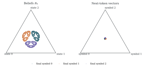
At a point , the three outgoing edges are obtained by applying and have probabilities given by the three coordinates of . Thus the three geometric copies visible at the next depth are also the three symbol-labelled branches of the belief-state automaton. 5. A belief and the observed symbol determine a unique updated belief , so the belief-state presentation is unifilar. The original generator is nonunifilar because its current hidden state and emitted symbol can leave several possible next hidden states. For the Simple Nonunifilar Source the reachable beliefs form a one-dimensional ladder, with each -edge resetting to . For Mess3 every symbol remains possible and the three update maps generate a rapidly branching, self-similar geometry. Finally, finite words form a countable set, so their image under the belief map is countable. Taking the closure adds limiting beliefs and can produce an uncountable fractal set.
Exercise 4.4 (Generalised hidden Markov models and predictive vectors). A -dimensional generalised hidden Markov model (GHMM) consists of a finite alphabet , real matrices , an initial row vector , and a column vector . Writing
these objects satisfy
for every and every .
(a) A probability law from matrix products. Consider
- Show that these quantities are nonnegative and that
for every . 2. Show that
Explain why this is the consistency condition needed to define a one-sided stochastic process. 3. The GHMM conditions do not require . Explain why the process need not therefore be stationary. Show that this additional equality is sufficient for stationarity.
(b) Predictive vectors. For any satisfying , define its predictive vector by
- Show that
and, for every continuation ,
- Derive the recursive update and identify its normalising factor:
- Conceptually contrast an HMM belief state with a GHMM predictive vector. Compare the meaning of their coordinates, their positivity and normalisation properties, and how they encode predictions of future observations.
(c) Predictive vectors need not be probability vectors. Consider the two-state HMM
Thus a hidden state is selected initially and thereafter emits a biased coin without changing state. Let
- Compute , and . Show that, for every ,
Deduce that this change of coordinates gives a valid GHMM for the same process. 2. Compute and . Verify directly from that
Explain why the entries of a GHMM predictive vector need not themselves be probabilities.
(d) The probability matrix and minimal dimension. For finite sets , define the probability matrix by
- Use the GHMM matrix product to factor as a matrix of prefix row vectors times a matrix of continuation column vectors. Deduce that
for every -dimensional GHMM realisation. 2. For the process in part (c), take . Compute and use an SVD to find its singular values. Deduce that the two-dimensional GHMM is minimal-dimensional.
Solution
(a)
- Nonnegativity is one of the GHMM assumptions. Expanding the product of the sum of the symbol matrices gives
Hence
where follows from . For this also says that the empty history has probability one. 2. Summing over the final symbol gives
Thus the length- distribution is the marginal of the length- distribution over its final coordinate, as required for a process indexed by . 3. The displayed GHMM conditions relate distributions at successive lengths but do not say that a block has the same distribution after shifting its time indices. If , then
The left side is , so the block distributions are invariant under a one-step shift. Iteration gives stationarity.
(b)
- The denominator in the definition is , and so
By the definition of conditional probability,
- Taking in part (i) gives
The first quantity is exactly the normalising factor in the update shown by the second equality. 3. An HMM belief state has coordinates , so they are nonnegative, sum to one, and refer to mutually exclusive hidden states. Predictive vectors are coordinates in a linear realisation: they need only satisfy and may have negative entries. Both summarise the history sufficiently to compute future-word probabilities through symbol-matrix products.
(c)
- Since
direct calculation gives
and
In particular , so , and . In a product, adjacent factors cancel:
The right side is an HMM sequence probability and is therefore nonnegative. All GHMM conditions are satisfied, and both realisations define the same process. 2. Both first-symbol probabilities are . Normalising gives
Moreover,
Hence
Although the second coordinate of is negative, all continuation probabilities obtained from it are valid. The predictive vector consists of coordinates in a chosen linear representation; unlike an HMM belief, its entries do not have to describe mutually exclusive hidden events.
(d)
- For and ,
Collecting the first factors as rows and the second factors as columns gives the requested factorisation through . The rank of the product is therefore at most . 2. The required probabilities are
Thus, in the order ,
It therefore has rank two. Every GHMM realisation must have dimension at least two, while part (c) supplies a two-dimensional realisation. It is minimal-dimensional.
5. Identifying belief geometry in transformers
So far, we have developed the conceptual framework of computational mechanics. We now ask whether neural networks trained for next-token prediction—including transformers and recurrent architectures—learn the predictive structures identified by that framework. You will read selected sections of two papers, then discuss their evidence and limitations in small groups.
Session at a glance
- Readings (75 minutes). Begin with the main reading and use the route below. Continue to the extension if time permits.
- Discussion (30 minutes). Form groups of three or four. Compare what you found convincing, confusing, or incomplete; use the prompts on page 2 if useful.
5.1 Readings
Prioritise the main reading. If you can answer its evaluation question, you have probably understood one of its central results. If time is short, skim the extension overview before deciding whether to continue.
5.1.1 [Main] Transformers represent belief state geometry in their residual stream
Reading route
- Skim. Sections 1, 2.1, and 2.2.
- Read. Sections 2.3 and 3–5.
- Evaluation. Explain Figure 6D. What do the comparison and shuffle control establish?
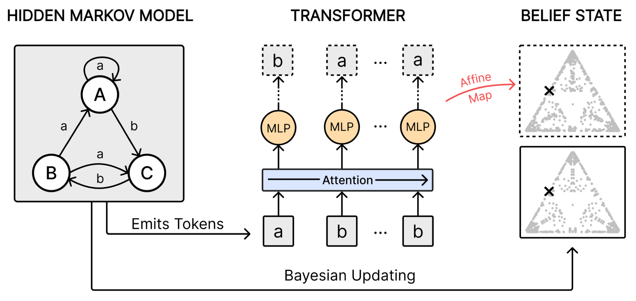
Overview. This paper presents evidence that transformers trained on HMM-generated sequences encode belief-state geometry in their residual streams. The claim is tested on the Mess3 and Random–Random–XOR (RRXOR) processes. For each process, the authors fit an affine map from residual activations to the exact HMM belief state and evaluate it using mean-squared error (MSE). The error decreases over training checkpoints. A shuffle control tests whether low MSE could arise merely because a high-dimensional activation space is being projected into a low-dimensional belief space.
5.1.2 [Extension] Neural networks leverage nominally quantum and post-quantum representations
Reading route
- Skim. Sections 1–3.
- Read. Sections 4–8.
- Evaluation. Explain Figure 3B. How are the light-blue and light-orange plots related to the corresponding dark-blue and dark-orange plots?
Overview. This paper extends the question from HMMs to generalised hidden Markov models (GHMMs). As in Part 3, a GHMM retains the matrix-product expression for output probabilities while relaxing the entrywise probabilistic constraints on its internal matrices. This larger model class can realise some processes in finite dimension even when a corresponding minimal HMM requires exponentially many more hidden states.
Using techniques related to those in the main reading, the authors study transformers, LSTMs, RNNs, and GRUs trained on processes with distinct GHMM and HMM realisations. Their results indicate that the networks learn belief-state representations associated with the lower-dimensional GHMM realisation. The finding suggests that neural networks can select among representational model classes in ways that capture dimensionality savings.
5.2 Discussion
Here are some prompts to consider:
- What is the most convincing evidence that transformers represent belief-state geometry? What is the least convincing?
- What additional experiment would most strengthen or weaken the claim?
- Which alternative hypotheses could explain the reported results?
- Can you explain each element of the diagram below—including the generative HMM, Bayesian updating, transformer activations, fitted affine map, and belief-state geometry?
6. Python exercises: HMM from scratch
The Python exercises are ARENA-style notebooks in two parts. Each part has an exercises notebook (with # YOUR CODE HERE stubs, inline tests, and collapsible solutions) and a fully worked solutions notebook.
- Part 1 — Sequence probabilities & next-token distributions (exercises) — Open in Colab
- Part 1 (solutions) — Open in Colab
- Part 2 — Belief states (exercises) — Open in Colab
- Part 2 (solutions) — Open in Colab
The Colab notebooks are self-contained: their setup cells write the helper modules into the session, so there is nothing else to install or download.
7. Learn more
- Beyond toy architectures – in-context learning
- LLMs have an amazing ability to adapt internal representations in-context – [Read: ICLR: In-Context Learning of Representations]
- LLMs can predict HMM data in-context – [Read: Pre-trained Large Language Models Learn Hidden Markov Models In-context]
- This suggests that internal representations of LLMs predicting GHMM data in-context, may resemble belief states.
- Processes consisting of GHMMs with richer structure [Read: Transformers learn factored representations]
- Review article of computational mechanics [Read: Between order and chaos]
- Simplex is a non-profit research organisation working on applying computational mechanics to AI safety.