Data Attribution
Which training examples caused a model to behave the way it does? These notes develop the main approaches to data attribution -- counterfactuals and Shapley values, classical and Bayesian influence functions, and training-dynamics unrolling -- with derivation exercises throughout.
By Louis Jaburi
Contents
- Introduction
- 1. Causality and Counterfactuals
- 2. Influence Functions
- 3. Bayesian Influence Functions
- 4. Unrolling
- 5. Practical Considerations and Open Problems
- 6. Further Readings
Introduction
Contents. These notes are structured as follows:
- Causality and Counterfactuals motivates the problem of data attribution through the lens of causal reasoning, exhibiting the shortcomings of naive counterfactual approaches.
- Influence Functions introduces the classical theory of influence functions for statistical models and discusses their translation to modern neural networks.
- Bayesian Influence Functions introduces susceptibilities and Bayesian influence functions, connecting them to the classical theory via a power series expansion.
- Unrolling presents the training-dynamics approach to attribution, deriving the basic formula and connecting it to influence functions in the appropriate limit.
- Practical Considerations and Open Problems discusses distributional versus single-model attribution, entangled latent concepts, and the distinction between similarity metrics and genuine attribution.
Prerequisites. We assume the following background, most of it standard for a machine-learning audience.
- Linear algebra: vectors, matrices, inner products, eigenvalues, quadratic forms, Hessians.
- Multivariable calculus: gradients, the chain rule, Taylor expansion, the implicit function theorem.
- Probability: expectations, conditional probability, Bayes' rule, Gaussian distributions.
- Deep learning basics: stochastic gradient descent, empirical risk minimisation, a standard supervised training loop.
Familiarity with the material from the singular learning theory tutorial (degeneracy, the local learning coefficient, posterior broadening) is useful but not required. We flag connections to the SLT day in remarks as they arise.
Fast-track. There is more material here than comfortably fits into a single day. Readers short on time may prefer one of the following routes; each is self-contained.
- From classical to modern influence functions. Skim Section 1 for motivation, then read Section 2 in full, including the derivation exercise.
- The Bayesian perspective. Read Section 2.1 for the influence function formula, then Section 3 in full. The connection exercise (Section 3.2) is the conceptual payoff.
- Training-dynamics attribution. Skim Section 2, then read Section 4 in full. The long exercise in Section 4.3 recovers the influence function as a limit of unrolling.
All three routes depend on the motivational material in Section 1. If reading only one section, read that one.
Acknowledgements. This tutorial was developed for the April 2026 Iliad Intensive and its template was inspired by the SLT day. Exercises and examples adapted from specific sources are credited inline.
1. Causality and Counterfactuals
1.1 Data attribution as causal analysis
At the heart of data attribution, we find a causal question: Which training examples caused a model to behave the way it does? If mechanistic interpretability aims for the causal analysis of a forward pass, data attribution aims for the causal analysis of a training run.1 Our north star is a decomposition of the training data into "causes" of the model's behaviour.
Two asymmetries between the two settings are worth keeping in mind from the start. First, both problems inherit the same conceptual difficulties of causal reasoning in general (explained in the next section) and there is no reason to expect data attribution to escape them. Second, a forward pass is cheap, while a training run is not. Where mechanistic interpretability can validate a claim by running many ablations, data attribution cannot in general afford even one retraining. That being said, there are also advantages: Generally speaking, the training process is more robust and the ablations we run may be more human understandable than high-dimensional modification of activations or weights.
Now, before developing such data attribution methods, we should be aware of the tension between causality and the ways we will validate a hypothesis. Finding a "true" causal relationship in practice can be much more difficult than it may seem at first glance. In the following section we take the question seriously, and find that the naive counterfactual answer fails in ways that matter.
1.2 Counterfactual attribution and its failures
The classical notion of causation is due to Lewis 1973: caused iff, had not occurred, would not have occurred. Applied to data attribution, this says that a training example "causes" a behaviour when removing it would have altered the behaviour, also known as the leave-one-out (LOO) counterfactual. We relax this definition from a binary to a gradual one.
Definition 1.1 (Counterfactual attribution). We attribute an action to a behaviour iff
- had occurred, would have occurred to a higher degree;
- had not occurred, would have occurred to a lesser degree (or not at all).
Definition 1.1 is the simplest formalisation of cause. But as Mueller 2024 emphasises, it breaks in at least two cases.
Overdetermination: redundant causes are missed. When two training examples are each sufficient to produce a behaviour, removing either one leaves the behaviour intact, and LOO attributes credit to neither.
Example 1.2 (Overdetermination in the bakery). OpenCroissant, a bakery, sources four ingredients: flour, butter, yeast, and sugar. Each can come from a standard or premium supplier. The bakery has observed that using all premium ingredients produces exceptionally fluffy croissants and wishes to identify which upgrades are responsible.
Unbeknownst to the bakery, exceptional fluffiness depends on two independent leavening mechanisms.
- Steam leavening. Premium butter has higher fat content and better water distribution, producing more steam and hence more lift.
- Biological leavening. A premium yeast strain ferments more vigorously, producing more gas and hence more lift.
Either mechanism alone causes exceptional fluffiness: puff pastry rises from steam alone, and bread rises from yeast alone. Downgrading premium butter to standard therefore has negligible effect on fluffiness (the threshold is still met), and likewise for yeast. Counterfactual attribution (Definition 1.1) concludes that neither butter nor yeast was a cause albeit both were.
The same pattern may arise in learning, where once a behaviour is learned, i.e. has hit saturation, additional examples will not affect it and appear as causally irrelevant.
Non-transitivity: counterfactuals do not chain. Direct ablation will not capture how an action causes a behaviour.
Example 1.3 (Non-transitivity of counterfactuals). The following scenario is due to Ned Hall, as reported in Hitchcock 2001.
(A) A hiker is wandering through the mountains when a boulder rolls down the hill.
(B) The hiker sees the boulder and dodges.
(C) The hiker is unharmed.
Counterfactually, (A) caused (B): had the boulder not rolled, the hiker would not have dodged. And (B) caused (C): had the hiker not dodged, she would have been crushed. But (A) did not cause (C): whether or not the boulder rolled, she ends up unharmed.
In the data-attribution setting this corresponds to chains of mediation. A training example may induce an intermediate feature, and that feature may drive a downstream capability, without the datapoint itself passing the counterfactual test against the capability end-to-end. Methods that look only at marginal effects miss the mediation.
1.3 Beyond leave-one-out: Shapley values
A natural response to overdetermination is to stop looking only at the LOO swap and instead ask how a training example contributes across all subsets of the training set it could be part of. This is the idea behind Shapley values (Shapley 1953).
Definition 1.4 (Shapley value). Let be a set function (a "game"). The Shapley value of element is
We can think of as a set of players and as the value of the coalition. In our previous example, the players are the premium ingredients and the value is the resulting fluffiness. Then will measure the fluffiness of the croissant when the ingredients in are premium and the rest are standard.
Shapley values partially address overdetermination. Returning to the baker example: in coalitions where neither butter nor yeast is premium, upgrading one has a large marginal effect; in coalitions where the other leavener is already premium, the marginal effect is small. Averaging gives each ingredient roughly half the credit.
Remark (Shapley still dilutes credit). Shapley values redistribute credit more fairly but do not fully solve overdetermination. Each of butter and yeast receives roughly half the credit for fluffiness, yet each alone is sufficient, so one could argue each deserves the full credit. Furthermore, Shapley values over a training set of size require evaluating on coalitions, each demanding a retraining. This is hopeless for realistic models.
1.4 Notation and goals
We close the section by fixing notation that will be used throughout.
- A training set is with .
- A model is a function parameterised by .
- The per-example loss is for some pointwise loss .
- We introduce a vector of data weights and define the weighted training loss
and we write for the unweighted loss.
- The behaviour we want to attribute is a differentiable scalar observable . This could be the loss on a held-out point, an average loss on a task, the logit of a specific completion, or any other scalar function of the trained parameters.
In general we want to know "If I change , how will this affect ?" This question is typically split into two parts:
- Parameter influence: "If I change , how will this affect the final parameters?"
- Influence on : "If I change the final parameters, how will this affect ?"
In practice we may think of the influence then as a measure of the composition of these maps
where we are intentionally vague about the first map and where the different approaches, influence functions, Bayesian influence functions, and unrolling, differ in how they interpret it.
That being said, all attribution methods in these lecture notes can be phrased as estimators of partial derivatives or finite differences of this map. The influence of an example is then computed as first-order approximation:
2. Influence Functions
In this section we develop influence functions: a closed-form, first-order approximation to the leave-one-out (LOO) counterfactual. The classical theory (Hampel 1974; Cook 1977) predates machine learning by decades. It was developed in robust statistics, where the question was which observations a parameter estimate is most sensitive to. For simple statistical models the answer is short: a single application of the implicit function theorem yields an inverse-Hessian-times-gradient formula whose factors have a clean operational interpretation.
The formula we arrive at then can be translated to the setup of neural networks, but its interpretation becomes unclear: The classical derivation assumes a unique global minimum and an invertible Hessian, neither of which holds for a neural network which is typically not trained to full convergence. We will see a partial fix for this issue in Section 2.2.
2.1 The influence function formula
Influence functions originate in robust statistics (Hampel 1974): given a statistical estimator, how much does it change when a single observation is added or perturbed?
Example 2.1 (Influence on the mean). Let be the mean of a distribution . If we contaminate by placing a fraction of its mass at a point , the new mean is
The rate of change at is : the influence of on the mean is simply how far is from the current mean. Observations far from the centre of the data move the mean the most.
We now translate this idea into the setting of Section 1.4, whose notation we use throughout. Recall that the weighted training loss defines a family of optimization problems parameterized by the weight vector . In the case of influence functions, we measure the influence of a data point on the optimal parameters
and we write for the trained parameters. We assume throughout this subsection that is the unique global minimum of and that the Hessian is positive definite, so that the implicit function theorem makes well-defined and smooth in a neighborhood of . In the notation of Equation 1 we set and Equation 3 yields then the following formula:
Definition 2.2 (Influence function). The parameter influence of training example at the trained parameters is
Under the assumptions above, the implicit function theorem gives (Exercise 2.1)
where is the Hessian of at . For any differentiable observable , the chain rule then yields the influence on :
Thus we get three components
- is the direction in parameter space along which pulls the optimizer.
- rescales this direction by local curvature: directions in which the loss is flat (small eigenvalue of ) get amplified, since a small force in a flat direction moves the minimum a lot.
- projects the parameter change onto the direction that matters for the observable .
In this section, we will focus on . The influence on any observable is obtained by computing the dot product .
Connection to leave-one-out. Setting (i.e., removing ) and applying the first-order Taylor expansion gives
i.e. the parameter influence is, to first order, the change in that would result from removing from the training set entirely.
Exercise 2.1 (Derivation of the influence function). Let as above and assume the Hessian is invertible. Recall that the implicit function theorem states: if is , , and the Jacobian at is invertible, then there is a unique map on a neighborhood of with , whose derivative is obtained by implicit differentiation of .
(a) Apply the implicit function theorem to to conclude that is well-defined and near . Which hypothesis of the theorem uses the invertibility of ? Where do we use that is the unique global minimum (rather than merely a critical point)?
(b) By differentiating the first-order optimality condition with respect to , show that
(c) Use the chain rule to obtain the formula for in Definition 2.2. Make sure to keep track of the evaluation at .
Solution
(a) Set . Then is in (assuming is ), and because is a critical point of the unperturbed loss. The Jacobian at equals , and the invertibility hypothesis of the implicit function theorem is exactly the assumption that is invertible. The theorem then yields a unique map on a neighborhood of with .
The uniqueness the implicit function theorem provides is only local: is uniquely defined as the critical point near . The assumption that is the unique global minimum is what lets us identify this local branch of critical points with the object we actually care about — the argmin. Without it, could jump to a different basin as varies, and the response function would fail to be continuous (let alone differentiable).
(b) Define the two-slot function
so that the optimality condition reads . The variable enters this identity in two places: once through the first slot via , and once directly through the second slot. The multivariate chain rule therefore produces two terms when we differentiate with respect to :
The two partials are:
- , which at equals the Hessian .
- : differentiating with respect to with held fixed picks out the single summand, giving .
Evaluating at and solving,
(c) For a differentiable observable , the chain rule applied to gives
where in the last step both factors are evaluated at , i.e. at .
Exercise 2.2 (Linear regression). Consider linear regression with training data , , and squared loss . Write . In this case the minimizer, the influence function, and the exact LOO update all have closed-form solutions. We will see that in general the influence functions can diverge in extreme cases.
(a) Derive the minimizer by setting . Show that .
(b) Compute the parameter influence from Definition 2.2.
(c) Define , so that is the unperturbed model and corresponds to fully removing . Using the Sherman–Morrison formula2, show that
where is the residual at and is the leverage of . Note that this is a rational function of . This is the ground truth effect of perturbing .
(d) Expand the closed form from (c) as a Taylor series in around the unperturbed point by recognizing as a geometric series, and obtain
Identify the term with the parameter influence from part (b), and observe that the higher-order terms () are suppressed by powers of the leverage .
(e) Specialize to the LOO endpoint . Sum the geometric series in to obtain the closed-form deletion update
The IF prediction is the leading term. Discuss the two regimes and : when does keeping only the linear term suffice, and when do all the higher-order corrections matter?
Solution
(a) The gradient of the training loss is . Setting this to zero gives , hence .
(b) The Hessian of the unweighted training loss is , and the gradient of the per-example loss at is . Plugging into Definition 2.2 with (so ),
a residual times a leverage-weighted input.
(c) The normal equations for read
or equivalently . Sherman–Morrison applied to the rank-one update on the left gives
where we write and . Multiplying through and using the identities and ,
the claimed expression. The result is rational in because the matrix being inverted is linear in .
(d) Expanding as a geometric series in (valid for ),
Reading off term by term:
- The term is , exactly the influence-function prediction — as it must be, since the IF is the linear coefficient of at .
- The term, , is the second-order Taylor correction. It carries one factor of leverage and is doubly suppressed: small both in and in .
- Each subsequent term picks up another factor of . The IF/LOO "error" is precisely this tail, viewed as a series in the perturbation size and the leverage.
(e) At the perturbation factor is unity, and the higher-order terms no longer have a small parameter in front of them — only powers of remain. The series collapses to a pure geometric series in :
The IF prediction is the leading term; everything else is the Taylor remainder. So the often-quoted "factor of " between IF and LOO is not a non-perturbative effect: it is the sum of all the higher-order Taylor terms, which OLS happens to admit in closed form because is rational. For more general M-estimators the response function is no longer rational and the higher-order terms do not sum to such a clean expression — but they are still there, with the same qualitative behavior.
In the two limiting regimes:
- (low leverage). Each higher-order term carries a factor of , so they are individually negligible and the IF approximation is essentially exact.
- (high leverage). The geometric series barely converges and the higher-order terms together carry an arbitrarily large total weight. The IF underestimates the true LOO change without bound.
This is a clean demonstration that even in a strictly convex, fully-converged setting the linearization in Definition 2.2 loses control over precisely the points one most wants to attribute — the ones the model could not fit without them. The lesson generalizes: high-leverage / outlier examples are exactly where IF approximations should be distrusted, and the modern fixes from Section 2.2 (damping, GNH, PBRF) all address related but more severe versions of the same issue.
Remark (What is leverage?). The quantity that appeared in Exercise 2.2 measures how unusual the input is relative to the bulk of the design. To see this, observe that is the empirical second-moment matrix of the inputs, so
is times a Mahalanobis-style squared norm of , taken in the metric defined by the data itself. Geometrically: directions that the data samples a lot correspond to large eigenvalues of and contribute little to , while directions that are barely sampled correspond to small eigenvalues of and so blow up under . Inputs that point in under-sampled directions get large leverage. High-leverage points are unusual in feature space.
Figure 1 illustrates the effect on a simple linear regression: removing a low-leverage point (A, near the bulk of the data) barely changes the fit, and the IF approximation is accurate. Removing a high-leverage point (B, an outlier on the -axis) changes the fit dramatically, and the IF underestimates the true LOO effect.
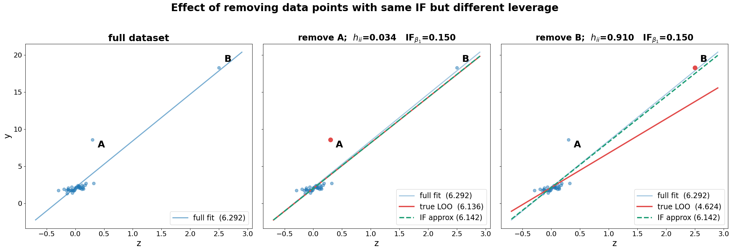
Influence approximation vs. LOO ground truth for a linear regression. Left: the full dataset. Centre: removing the low-leverage point A () barely perturbs the fit; the IF prediction closely matches LOO. Right: removing the high-leverage point B () moves the regression line substantially; the IF underestimates the true change. Note that both points have the same parameter influence.
2.2 Translation to modern neural networks
The derivation in Section 2.1 relied on two assumptions:
(i) is the unique global minimum of the training loss;
(ii) the Hessian is positive definite.
While neither holds for a modern neural network, the quantities in Definition 2.2 are, in principle, computable. Koh & Liang 2020 popularized the influence function formula as a tool for deep learning, and a substantial body of work has tried to make it useful at scale.
(1) Non-uniqueness and a singular Hessian. For a neural network the global minimum is usually not unique. The set of minimizers is generically a positive-dimensional zero locus, and the Hessian at any point on it is singular: it has a nontrivial null space corresponding to directions of parameter movement that leave the loss unchanged. This is the degeneracy phenomenon observed in the SLT day, and it means we cannot invert as in Definition 2.2.
The standard remedy is to dampen the Hessian: replace with for some . This is the same as adding an -regularizer to the training objective ; this yields a new loss function .
(2) Negative curvature. Even after damping away the zero eigenvalues, at a non-converged checkpoint can have negative eigenvalues, in which case may still be ill-conditioned or even point in the wrong direction. The standard fix is to replace with the Gauss–Newton Hessian (GNH)
where is the parameter-output Jacobian and is the Hessian of the per-example loss with respect to the network outputs (not the parameters). For the cross-entropy and squared losses is positive semidefinite, hence so is . The GNH is a local approximation to the true Hessian that ignores second derivatives of the network outputs with respect to the parameters. It is not hard to show that and differ by a term that vanishes at a critical point of , so the GNH is a reasonable proxy for when is close to optimal.
(3) Non-converged checkpoints. In practice is not a critical point of . The classical formula in Definition 2.2 is then evaluated at a point where .
The fix proposed by Bae et al. 2022 is to replace the original training loss by a surrogate for which is optimal by construction. Concretely, define the proximal Bregman objective (PBO) as
where is the Bregman divergence of the output-space loss around . The first term penalizes any change in the network's predictions on the training set, with the current model as the reference; the second is the perturbation of interest; the third is the damping. By construction, is the minimizer of regardless of whether it is a critical point of the original loss. The minimizer of for nearby defines the proximal Bregman response function (PBRF).
When one re-derives the influence function formula starting from instead of , the result is
the same expression that the modern literature uses. This is effectively the counterfactual it approximates. As Bae et al. 2022 put it: if influence functions are the answer, the question is the PBRF, not LOO retraining. We refer to their paper for a detailed decomposition of the remaining gap between the PBRF and the original LOO counterfactual.
Remark (Connection to the SLT day). A central obstacle to the application of influence functions to modern neural networks is degeneracy: the set of minimizers of an overparameterized model is singular and the Hessian has a large null space. In Section 3 we will see a degeneracy-aware alternative: Bayesian influence functions, which replace inverse-Hessian computations with covariances over a localized posterior.
Remark (Scaling and EK-FAC). Even with the PBRF reframing, computing for a billion-parameter model is not directly feasible. Grosse et al. 2023 scale influence functions to large language models by approximating with EK-FAC (a Kronecker-factored approximation to layerwise curvature).
Exercise 2.3 (Failure of the first-order approximation in a degenerate model). Consider the toy two-parameter model from the SLT lecture day in which enters the loss only through the product , with squared loss on training data .
(a) Write down the Hessian of the training loss at any minimizer with . Show that it has rank one, and identify the one-dimensional null space geometrically.
(b) Compute the influence function for the observable , treating as a Moore–Penrose pseudoinverse3. How does it compare with the exact LOO change in ?
(c) Repeat (b) using the damped inverse for a small . Discuss how the answer depends on , on the choice of minimizer along the singular set, and on . What does this say about the proximity gap?
Solution
(a) The per-example loss is . Its second derivatives are
Summing over and evaluating at any minimizer with ,
where we used for the off-diagonal. This is rank one, with image .
The null space is . Geometrically: the minimizers form the hyperbola , and the tangent to this hyperbola at is exactly the direction — the infinitesimal generator of the rescaling symmetry at . The null space of is the tangent to the manifold of minimizers.
(b) We need two gradients at the minimizer. For the observable :
For the per-example loss at :
Both point in the direction — neither has a component in the null space of . The Moore–Penrose pseudoinverse of is
Plugging into the IF formula,
The factors cancel: the pseudoinverse IF is independent of the choice of minimizer .
Comparison with exact LOO. Removing changes the sample mean to , and the observable at any new minimizer is . So the exact LOO change is
The IF predicts . The ratio is with leverage — every point has equal leverage in this one-effective-parameter model, and we recover the same correction as in Exercise 2.2.
(c) The eigenvalues of are (eigenvector ) and (eigenvector ). So
Since and both lie in the direction, the term does not contribute, and
Dependence on the minimizer. For the answer depends on , which varies along the orbit . For instance, the "balanced" minimizer gives , while the "unbalanced" choice gives . Different minimizers yield different IFs. This is the proximity gap: the damping term breaks the rescaling symmetry and anchors the computation at a particular point on the orbit.
Limit . regardless of , recovering the pseudoinverse answer from (b). The damping-induced dependence on the minimizer vanishes.
Limit . : heavy damping kills all attribution, because the proximal penalty makes it too costly to move at all.
The punchline: for this particular observable (, which is constant along the orbit), the pseudoinverse gives a clean, minimizer-independent answer and the damping only introduces a spurious dependence. But for an observable that does vary along the orbit — say — would have a component in the null direction , the term would contribute, and the IF would diverge as . In that case damping is not a nuisance but a necessity, and the choice of minimizer genuinely matters. This is the core tension of the proximity gap: it is a distortion for orbit-invariant queries, but a regularizer for orbit-dependent ones.
3. Bayesian Influence Functions
Classical influence functions give a first-order approximation to the change in a point estimate when the training data is perturbed. The Bayesian reformulation replaces this point estimate by a distribution over parameters: if we perturb the training data, how does our posterior over the parameter space change? This leads naturally to the Bayesian generalization of influence functions introduced in Kreer et al. 2026. In the setting of Equation 1 we set not to be a single weight, but a whole distribution over parameters , namely the posterior.
Susceptibilities. The Bayesian influence function is one instance of a more general object studied by Baker et al. 2026. Given a tempered Gibbs posterior at inverse temperature , any pair of observables defines a susceptibility
The differentiation argument we will apply in Exercise 3.1 shows in full generality. Taking gives the Bayesian influence function developed below. Other choices of yield other sensitivity notions, see e.g. the refined learning coefficients (Baker et al. 2026, Appendix D.2). We will not need the general framework again; we mention it only to locate the BIF within the wider susceptibility family.
3.1 Bayesian influence functions
We now specialize the susceptibility story to data attribution. Instead of asking "how does change when we perturb the training weights?" (Definition 2.2) we ask "how does change?" The answer turns out to be remarkably clean: the derivative becomes a covariance, and the Hessian inversion of the classical formula is replaced by posterior sampling.
The tempered posterior. Given training data with per-sample losses , sample weights , and a prior , define the tempered posterior
When and the loss is a negative log-likelihood, this is the standard Bayesian posterior. When the losses are not log-likelihoods, is a Gibbs measure; the mathematics is identical.
Definition 3.1 (Bayesian influence function). The Bayesian influence function (BIF) of training example on the observable is the derivative of the posterior expectation of with respect to the sample weight :
The definition is the natural Bayesian analogue of Definition 2.2: replace with . The following exercise shows that this derivative has a clean closed form. Recall that for two real-valued random variables and defined on the same probability space, the covariance is
When and are functions of the random parameter , we write to indicate that the expectation is taken over the posterior . If is vector-valued (), the covariance is the vector whose -th entry is .
Exercise 3.1 (The BIF is a covariance). Let be the tempered posterior of Equation 8 and write for the unperturbed posterior. By differentiating with respect to , show that
Hint: Write and differentiate the ratio using the quotient rule. The key identity is .
Solution
Write for the normalizing constant, so that
Differentiating with respect to and applying the quotient rule:
The first term is . For the second, , so it equals . Evaluating at :
Structurally: in the classical IF, the "correlation" between and is mediated by the inverse Hessian acting on their gradients at a point; in the BIF it is mediated by the full posterior distribution. The inverse Hessian is how a Gaussian posterior would produce a covariance (as we will see in Exercise 3.2), so the BIF strictly generalizes the classical formula.
Remark (Statistical physics). The identity is a standard fluctuation–response relation in statistical physics: the response of an observable to a change in an external field equals the covariance of that observable with the conjugate energy.
Localization. Computing expectations over the global posterior is generally intractable for neural networks, and we are typically interested in the behavior of a specific trained checkpoint , not a global Bayesian average. Following Kreer et al. 2026, we localize the posterior by adding a Gaussian penalty centered at :
where is a localization strength that controls how tightly the posterior concentrates around . The local BIF is then
where denotes covariance under . We will see in Exercise 3.2 that the localization parameter plays exactly the role of the damping parameter in the PBRF formula (6).
Practical computation via SGLD. The local BIF requires estimating a covariance under . This is done by drawing samples from using stochastic gradient Langevin dynamics (SGLD), which adds calibrated Gaussian noise to SGD updates:
where , is a mini-batch of size and is the step size. After a burn-in period, the iterates are approximately distributed according to , and the covariance in (11) is estimated by the sample covariance of across draws. Running multiple independent chains from improves coverage.
Example 3.2 (Bayesian linear regression). Take the linear regression setup of Exercise 2.2 with a Gaussian prior added. The posterior is conjugate: with and . A direct Gaussian-moment computation applied to (9) with the observable gives
where is the posterior-mean residual and . This is the damped influence function with the damping parameter equal to the ratio of observation noise to prior variance. In the flat-prior limit we have , , and we recover the classical IF of Exercise 2.2.
3.2 Exercise: Connecting Bayesian and classical influence functions
As we have seen in the SLT day, tools involving the Hessian are usually a low-order approximation of an expansion. This is also true for influence functions: In the non-degenerate case the classical IF is the leading-order term of the BIF under a Laplace approximation. The following exercise makes this precise by computing a power series expansion of the BIF covariance and identifying the classical IF as the leading-order term. The argument follows Kreer et al. 2026, Appendix A.
Exercise 3.2 (Power series expansion of Bayesian influence functions). Let be a local minimum of the training loss with positive-definite Hessian . Write , and abbreviate , for the gradient and Hessian of the observable, and , for the per-sample loss.
(a) (Laplace approximation.) Consider the posterior . Taylor-expand to second order around , using the fact that at a minimum. Argue that for large the quadratic term in dominates the prior , and conclude that
Under this approximation, . (This is called the Laplace approximation; the Bernstein–von Mises theorem guarantees it is asymptotically exact for non-singular models.)
(b) (Taylor expansion of the covariance.) Expand and in Taylor series around :
Using the fact that constant terms drop out of covariances and that where denotes the -th order term in the Taylor expansion of , show that the BIF decomposes as
Why do terms with odd vanish?
(c) (Leading order: classical IF.) Compute the term:
Conclude that is the classical influence function from Definition 2.2. This is the leading-order term of the BIF.
(d) (Second-order correction.) Compute the term using Isserlis' theorem (the Gaussian moment identity with ). Show that
This correction involves the Hessians of the observable and per-sample loss. It captures second-order curvature interactions that the classical IF misses entirely. In the linear regression setting of Example 3.2, why does this correction vanish?
(e) (Localized version: damped IF.) Now consider the local BIF of Equation 11 with localization strength . The localized posterior is approximately . Repeat the leading-order computation of part (c) to show that
This is precisely the damped influence function of Equation 6, with the localization strength playing the role of the damping parameter . The local BIF is thus a natural, higher-order generalization of the damped IF: it agrees at leading order and includes all the corrections from parts (b)–(d) with replaced by .
Solution
(a) The log-posterior is . Taylor-expanding around the minimum :
The linear term vanishes because is a critical point. Substituting into :
Since , the Hessian scales as , while the prior contributes to the log-density. For large the quadratic term dominates, giving . This is the Laplace approximation. (The Bernstein–von Mises theorem makes this rigorous: under regularity, the posterior converges to this Gaussian in total variation as .)
(b) Since for any constant , the constant terms and drop out. The covariance of the two Taylor series is bilinear, so it distributes over the sum of terms:
Under , is a degree- polynomial in . The covariance involves moments of of degree . For a centered Gaussian, odd moments vanish: when is odd. If is odd, then all moments in and involve an odd total degree, so both vanish and .
(c) and are linear in . Their covariance is
Negating gives , which is the classical influence function from Definition 2.2.
(d) Write and . We need with , .
For the expectation: and .
For the cross-moment: . By Isserlis' theorem:
The first pairing gives , which cancels in the covariance. The other two pairings each give (by cyclicity of the trace and symmetry of , , and ). So
In the linear regression setting with (a coordinate function), : the observable is linear in , so its Hessian vanishes and the entire correction is zero. This is why the BIF equals the (damped) IF exactly for linear regression — all corrections beyond leading order involve or higher derivatives of , which vanish for a linear observable.
(e) The localized posterior of Equation 10 has effective Hessian , so the Laplace approximation gives . The leading-order computation from part (c) becomes
which is the damped IF of Equation 6 with in the role of . The higher-order corrections from parts (b)–(d) carry through with replaced by throughout.
(f) Summary: For regular (non-singular) models, the posterior is approximately Gaussian (Bernstein–von Mises), the Taylor expansion converges, and the term dominates (it scales as while higher terms scale as and beyond). The classical IF is a good approximation because it is the leading term. For singular models (neural networks), the posterior is concentrated on a positive-dimensional variety, not at an isolated point. The Laplace approximation fails: the Hessian has a large null space, the posterior is non-Gaussian, and the Taylor series does not converge around . In this regime, the BIF — defined as an exact covariance under the true posterior — captures the full geometry, while the classical IF is at best the leading term of an expansion that does not converge. The BIF is the fundamental object; the IF is the Gaussian shadow it casts.
Remark. We conclude that the classical (damped) IF is the leading term of the (local) BIF under a Laplace approximation. For non-singular models with enough data, the Laplace approximation converges and the higher-order terms are small. But for singular models (neural networks), the Laplace approximation fails, the posterior is not Gaussian, and the BIF captures geometry that the classical IF cannot see.
3.3 Long Exercise: Influence functions as optimal linear transport
The previous exercise showed that the classical IF is the leading-order term of the BIF under a Laplace approximation. We now take a different perspective, due to Mlodozeniec et al. 2025: instead of asking "what does the BIF reduce to?" we ask "what is the best way to shift the parameters to approximate the effect of a data perturbation?" The answer turns out to be: the influence function, and its optimality does not require the Laplace approximation to hold.
Setup. Let denote the total training loss, and abbreviate for the per-sample loss at example . Define the Boltzmann distributions at inverse temperature :
so that is the Boltzmann distribution after downweighting sample by . The low-temperature limit concentrates on the set of global minima .
Now suppose we want to approximate the effect of the perturbation without resampling from . The simplest approach is to take each parameter drawn from and shift it to for some smooth vector field . If is chosen well, the distribution of the shifted parameters should be close to . The question is: what is the optimal ?
To make this precise, we need to know the density of the shifted parameters. If and we set , then by the multivariate change-of-variables formula, has density
where is the Jacobian matrix of and the denominator is the usual volume-change factor.4 We measure how well approximates by the KL divergence . Rather than computing this directly, it is cleaner to write it as an expectation over the original distribution :
This identity follows by substituting (12) into the definition of KL and changing variables back to . We define the asymptotic KL cost
The normalization kills the determinant term (which is ) and the entropy terms, isolating the energy contribution (which is ).
Exercise 3.3 (Influence functions as optimal parameter shifts). Let be a non-degenerate minimum of with positive-definite Hessian . In this exercise we work at the unique minimum, so the limit simply evaluates everything at .
(a) (KL in terms of energies.) Starting from (13), substitute and , and show that
where . Explain why the last two terms vanish in the limit. Hint: , and by Laplace's method .
(b) (Taylor expansion at .) Since the expectation under concentrates at as , expand and using :
Similarly, show that , by minimizing the Taylor expansion of around . Combine everything to obtain
Hint: After substitution, the terms that do not depend on should assemble into and cancel with the partition-function contribution, leaving a perfect square.
(c) (IFs are optimal.) The cost (15) is a squared Mahalanobis distance (in the Hessian metric) between the shift and the influence function . Conclude that the IF minimizes to among all smooth shift maps , and that the minimum cost is .
State the result in words: the influence function is the approximately KL-optimal way to shift the parameters of the unperturbed Boltzmann distribution to approximate the perturbed one.
(d) (Degenerate case.) Now suppose lies on a minimum manifold and is singular with null space . Argue (without detailed proof) that:
- The cost (15) generalizes to , where is the Moore–Penrose pseudoinverse.
- The minimizer is for any : directions in the null space of have zero cost, because the Hessian assigns zero curvature to movement along the minimum manifold.
- The IF (with pseudoinverse) is therefore optimal for the directions that matter, but the component of the shift along the flat directions is unconstrained.
Connect this to the SLT perspective: for singular models, the minimum is a variety, and the IF tells you how to move off the variety but is silent about movement along it.
(e) (Linear regression check.) Specialize to the Bayesian linear regression setting of Example 3.2 with prior . The Boltzmann distribution at inverse temperature is the Bayesian posterior , which is already Gaussian, no need to take . A constant shift sends to . The true perturbed posterior (downweighting by ) has mean and covariance . Using the KL formula for Gaussians with the same covariance, show that
which is minimized at . Verify that this is consistent with (15): the "Hessian of the energy" (training loss plus prior) is , and .
(f) (Comparison with Exercise 3.2.) The Laplace expansion exercise and this exercise both relate the IF to the BIF, but they answer different questions:
- Exercise 3.2 is an algebraic identity: BIF IF higher-order corrections. It requires the Laplace approximation (hence non-singular , Gaussian posterior) and tells you what happens when you truncate the BIF.
- This exercise is an optimality result: the IF shift minimizes the KL divergence between the shifted and true perturbed distributions. The result (parts a–d) needs only mild regularity of and works even for singular (via the pseudoinverse).
Summarize: the Laplace expansion tells you what the IF is (the leading Gaussian term of the BIF). The optimality perspective tells you why it works (it is the best first-order correction to the parameter distribution). The second viewpoint does not require the posterior to be Gaussian, which is why Mlodozeniec et al. 2025 argue that it provides a better explanation for the empirical success of IFs in deep learning.
Solution
(a) Using and , substituting into (13) gives
Dividing by and rearranging gives the claimed expression. As : (i) since the log-determinant is (bounded for smooth and small ); (ii) by Laplace's method, , so , which is a constant independent of ; (iii) the expectation concentrates on .
(b) At , , so the Taylor expansion of starts at the quadratic term: . For : . Combined:
For the infimum: expanding to second order in and minimizing, the optimal perturbation is , giving
So .
Adding the two contributions:
Completing the square: , since expanding the right side gives .
(c) Since is positive definite, the squared Mahalanobis form with equality iff . At the minimum, : the IF shifts the distribution with only a third-order KL residual. Any other shift incurs a strictly positive cost proportional to its Mahalanobis distance from the IF. The IF is the unique optimal shift among all smooth vector fields , not just among constant maps.
(d) When is singular, the quadratic form is zero for : movement in the null space has zero Hessian cost because the loss is flat along the minimum manifold. The pseudoinverse inverts only the non-degenerate directions, and the completed square becomes . This vanishes whenever , i.e., the minimizer is for any .
Geometrically: the IF determines the optimal shift off the minimum manifold (perpendicular to ), but movement along is invisible to the energy at this order. In the SLT language: the degeneracy of the singular set means that many shifts are equally good at leading order — the IF picks one, but the null-space ambiguity is real.
(e) For linear regression with Gaussian prior, the posterior is with . A constant shift sends to . The true perturbed mean is with . For two Gaussians with the same covariance:
This is minimized at . To check consistency with (15): the "Hessian of the energy" in the Boltzmann distribution is , and . The general formula (15) reduces to , exactly as computed directly.
(f) The two exercises are complementary:
- The Laplace expansion (Exercise 3.2) tells you what the IF is: the leading-order term of the BIF covariance under a Gaussian approximation to the posterior. The higher-order corrections (Hessian products, etc.) are visible but require the Laplace approximation to hold.
- The transport perspective (this exercise) tells you why the IF works even when the Laplace approximation fails: it minimizes the KL cost of transporting the parameter distribution, and this optimality holds in the limit under mild regularity assumptions — no Gaussianity required. For singular models, the pseudoinverse handles the degenerate directions naturally (part d), and the result still says: the IF is the best you can do with a smooth first-order map.
This provides what Mlodozeniec et al. 2025 call a "distributional" justification for IFs in deep learning. The original justification (implicit function theorem, convexity) does not hold for neural networks. The Laplace/BIF justification (Exercise 3.2) requires Gaussianity of the posterior, which also fails. But the transport optimality result asks only for bounded derivatives and a well-defined minimum — conditions much closer to what actually holds in practice.
Remark (Optimal transport). In the language of optimal transport, the map is called a transport map, and the distribution of the shifted parameters is its pushforward, written . The cost functional is the asymptotic KL divergence between the pushforward and the target. Exercise 3.3 then says that the influence function is the KL-optimal transport map from the unperturbed to the perturbed Boltzmann distribution, at first order in . This is the perspective developed in Mlodozeniec et al. 2025, who prove a more general version (their Theorem 3) that applies to all smooth diffeomorphisms, not just maps of the form .
4. Unrolling
The influence functions of Section 2 and the Bayesian influence functions of Section 3 both have something in common: they analyze the endpoint of training, not the dynamics that led to it. Under the assumptions of the unique global minimum, this is not a problem: the training trajectory is irrelevant, since all roads lead to the same outcome. But in practice the training path will matter a lot. Ultimately, we are studying generalization and this is ultimately a question about the training dynamics. Similarly, the BIF looks at the posterior expectation shifts. To give a concrete failure mode: a training point that appears in the first mini-batch of the first epoch will have a very different effect compared to the same point appearing towards the end of training.
If we write down the training trajectory as a composition of -dependent maps:
where each is one optimizer step (a gradient step, an Adam update, etc.): , we can observe an analogy to a forward pass through a neural network:
where each is one layer: .
| **Forward pass ** | Training trajectory | |
|---|---|---|
| Inputs | Model weights | Data weights |
| Intermediate states | Activations | Parameters |
| Output | Loss | Observable |
| Differentiation method | Backpropagation | Unrolling |
Data attribution via unrolling is to a training run what backprop is to a forward pass: differentiating a composition of maps to identify which inputs matter most.
This invites the following question: Can we backprop through the training trajectory? The gradients with respect to the then indicate which data points would need to be up- or downweighted to change the final observable . And in principle, we can! We can differentiate through the training computation, step by step, treating the final parameters as an explicit function of every gradient update along the way. The result is a chain-rule expression that decomposes data attribution into per-step contributions and naturally incorporates the optimizer, learning rate schedule, mini-batch ordering, and training duration. We will derive the unrolling formula similar to the backprop formula for a forward pass, and then discuss two approaches to making it practical: one that materializes Jacobians and one that computes Jacobian-vector products implicitly. In the setup of Equation 1 we take , the final checkpoint of the training run.
4.1 The training-dynamics approach to attribution
We fix notation for the training process. Given a dataset with sample weights , the optimizer runs for steps. At step , a mini-batch of size is drawn, and the parameters are updated by
where is the learning rate at step . At this is ordinary SGD on the unweighted loss. The initial parameters are independent of . For simplicity we can assume that we are training for one epoch only, so that each example appears in exactly one mini-batch, but the formulas hold more generally.
The counterfactual. We want
the sensitivity of a final-model observable to an infinitesimal change in the weight of training example .
4.2 The unrolling formula
Central to computing the data weight gradient is the Jacobian of one SGD step with respect to the current parameters. Define
where is the mini-batch Hessian at step . The Jacobian of the map from step to step is the ordered product
Similarly, the direct effect of at step (when ) is the per-example gradient:
The full derivative is obtained by chaining direct effects through remaining steps:
Each term in the sum corresponds to one training step in which appeared in the mini-batch: it is the gradient of at the parameters of that step, propagated forward through the Jacobians of all subsequent steps.
The influence on an observable follows by the chain rule:
Remark (Which questions does unrolling answer?). Equation (20) looks like a sum over training steps and, for a fixed realization of the mini-batch sequence, it is a deterministic chain-rule computation. But the training run has randomness (initialization, mini-batch ordering, data augmentation), and so does the counterfactual: if we change , the mini-batch sequence might be the same or it might differ. Unrolling as written differentiates through a specific training run: it answers the single-model attribution question, "how would this particular training trajectory have ended differently?" The distributional question, which looks at the expected change over random training, would require averaging (20). This distinction, which we will revisit in Section 5, is the training-dynamics analogue of the single-posterior-mode vs. full-posterior distinction in Section 3.
Exercise 4.1 (Derivation of the unrolling formula). (a) Starting from the SGD update (16), apply the chain rule to write as a sum of two terms: one from the explicit dependence on (the direct effect) and one from the dependence of on (the indirect effect). Show that the result is the recursion
with initial condition . Compute the Jacobian explicitly in terms of the mini-batch Hessian which leads to (17).
(b) Solve the recursion by "unrolling" it (i.e. by substituting repeatedly and using (18)) to obtain (20).
(c) (Preconditioned SGD.) Suppose instead that the optimizer uses a preconditioner :
This includes momentum-free Adam and natural gradient methods as special cases (with appropriate ). Show that the step Jacobian becomes and that the unrolling formula generalizes to
where . The only change is that each gradient is premultiplied by the preconditioner at the step where it appears. What does this say about the effect of using Adam vs. SGD on the attribution of a data point that appears early in training?
Solution
(a) Differentiating (16) with respect to at via the chain rule:
The initial condition is since does not depend on .
(b) Substituting the recursion repeatedly:
where the last step follows from killing the term. This is (20).
(c) With the preconditioned update (22), the indirect effect picks up the preconditioner in the Hessian term: . The direct effect becomes . Unrolling the recursion as in (b) gives (23). The preconditioner at step acts as a local rescaling of the gradient: Adam's adaptive scaling amplifies gradients in directions with historically small second moments. A datum appearing early in training (when Adam has not yet accumulated accurate statistics) will have its gradient rescaled differently than the same datum appearing later, when has stabilized. This is a concrete mechanism by which optimizer choice affects per-datum attribution.
Remark (TracIn). Pruthi et al. 2020 observed that the Jacobian products in (20) are both the most expensive and the most unstable part of the computation. Their method, TracIn, simply drops them, setting :
where is a set of checkpoints (typically one per epoch).
There are two ways to make (20) practical. The first is to compute the Jacobian products explicitly, or rather an approximation thereof. The second is to avoid materializing Jacobians altogether and instead compute Jacobian-vector products implicitly by reverse-mode automatic differentiation through the training loop. We will discuss both approaches in turn.
4.2.1 Materializing the Jacobian
In this subsection we will derive the SOURCE method (Bae et al. 2024), which introduces a small number of approximations of Jacobians that reduce the full unrolling computation to something resembling an influence-function calculation at each of several checkpoints.
Stationary segments. Divide the training steps into segments at checkpoints , and let be the number of steps in segment . Within each segment, make the stationarity approximation: the expected mini-batch Hessian and per-example gradient are approximately constant,
Similarly, write for the average learning rate in segment .
Segment Jacobian. Under the stationarity approximation, the product of step Jacobians within segment simplifies to a matrix power:
The matrix exponential is well approximated by the matrix power when has small spectral norm. In an eigenbasis of with eigenvalue , the segment Jacobian acts as the scalar filter : high-curvature directions ( large) are exponentially damped, while low-curvature directions ( small) are preserved.
Segment response. Return to the unrolling formula (20) and restrict the sum to the steps inside segment . The contribution of datum during this segment is
where the Jacobian propagates each gradient contribution forward to the segment boundary (propagation from to the end of training is handled by the inter-segment Jacobians in the full formula below). Now apply the stationarity approximation: replace each by , each learning rate by , replace the indicator by its expectation (datum appears in a random batch with probability ), and use the segment Jacobian approximation . This gives
The sum is a matrix geometric series. Using with and passing to the matrix exponential:
To understand this, work in an eigenbasis of . On an eigenvalue , the matrix acts as the scalar
Note the similarity to the classical influence function formula, which applies (the inverse Hessian eigenvalue), and with the damped IF (6), which applies . Thus can be seen as a principled damping constant:
- Large (directions the optimizer has fully converged along): , so . Agrees with the classical IF.
- Small (directions the optimizer has barely moved along): , so . A finite constant, not .
- Crossover at : directions with curvature below this threshold are automatically suppressed.
Full formula. Chaining the segment Jacobians and responses across all segments:
where the product is ordered with on the left. With a single segment (), the formula reduces to , which is the classical IF with replaced by the filter .
Remark (Unrolling provides a principled damping). The crossover in the filter plays exactly the role of the damping parameter in the PBRF formula from Section 2.2, but it is not a free parameter. It is the reciprocal of , the total training effort (learning rate number of steps) in the segment. Directions that the optimizer has not had time to converge along are automatically down-weighted, because the Jacobian products have not had enough steps to amplify them. The practical consequence: the damping that influence-function methods require careful tuning of has a natural value determined by the training process, and unrolling recovers it without any tuning.
4.2.2 Implicit JVPs and the REPLAY algorithm
The second approach to evaluating (20) avoids materializing Jacobians altogether. Instead, it uses reverse-mode automatic differentiation through the training loop, computing Jacobian-vector products (JVPs) implicitly. This is the strategy of the MAGIC method (Ilyas & Engstrom 2025), building on the metagradient framework of Engstrom et al. 2025.
Setup. Model the entire training process as a composition of differentiable update functions:
where is the full optimizer state at step (parameters, momentum buffers, etc.), is the weighted mini-batch gradient, and is the optimizer's update rule (SGD, Adam, etc.). The attribution target is , which depends on through the entire chain of updates.
The metagradient decomposition. Applying the chain rule through this composition:
The vector is the sensitivity of the final observable to the state at step ; it satisfies the backward recursion
This is just backpropagation through the training loop. The vector is the direct effect of at step : it captures how the gradient at step depends on the data weights. For vanilla SGD, reduces to .
REPLAY: efficient reverse-mode through training. The backward recursion (33) requires the optimizer state at every step. Naively this means storing all states, which is prohibitive for long training runs. The REPLAY algorithm (Engstrom et al. 2025) solves this with a hierarchical checkpointing scheme:
- Save evenly-spaced checkpoints along the training trajectory.
- When the backward pass needs a state between two checkpoints, replay the training forward from the nearest saved checkpoint to regenerate it.
- Apply this strategy recursively (a -ary tree of depth ).
The result is exact (to floating-point precision) differentiation through all training steps, using stored states and total forward-pass work, a logarithmic overhead over the cost of training itself.
Comparison with explicit unrolling. The implicit approach has two main advantages:
- Exactness. No stationarity or matrix-exponential approximations are needed; the Jacobian-vector products are computed exactly by autodiff.
- Generality. Any differentiable optimizer (Adam, LAMB, etc.) and any training pipeline (multi-stage, curriculum learning) are handled transparently, since is just a function.
The price is computational: REPLAY requires training-equivalent steps and careful engineering of the checkpointing schedule, whereas the explicit approach requires only a handful of checkpoints and an EK-FAC-style Hessian approximation at each. The choice depends on the scale: for moderate-size models where replaying training is feasible, MAGIC gives exact answers; for large-scale models where even one extra training pass is expensive, the SOURCE approximation with – segments may be the only practical option.
4.3 Long Exercise: From unrolling to influence functions
The unrolling formula (20) and the influence function (6) appear to be very different objects: one is a sum over training steps of Jacobian-propagated gradients, the other is a single inverse-Hessian-times-gradient computation at the endpoint. The following exercise shows that, in the right limit, unrolling converges to the classical influence function. The key observation, due to Mlodozeniec et al. 2025, is that the joint process , where is the unrolling response, forms a Markov chain, and its limiting behavior can be analyzed with standard stochastic-approximation tools. This yields a convergence result that requires only that SGD reaches a local minimum, not that the loss is convex.
Exercise 4.2 (Convergence of unrolling to influence functions). Consider the SGD update with an interpolated loss that downweights example by :
so is the original training run and corresponds to removing . Define the response .
(a) (The response recursion.) By differentiating (34) with respect to at , derive (35), where is the step Jacobian from (17). The top row is ordinary SGD; verify that the bottom row is the same recursion as Exercise 4.1(a), but now with stochastic batches. Since the driving terms depend only on and the i.i.d. batch selection , the joint process is a Markov chain. Why is this observation useful?
(b) (Deterministic warm-up: full-batch GD.) As a warm-up, consider full-batch gradient descent with constant learning rate (i.e. for all ). Assume training has converged: and for all in a window of length . Show that the response over this window satisfies
Hint: Sum the geometric series using the identity .
Take (assuming ) and recover the influence function .
(c) (Stochastic case: convergence to IF.) Now return to SGD with i.i.d. batches and a decaying learning rate satisfying , (the Robbins–Monro conditions). Assume SGD converges to a local minimum with positive semidefinite. The continuous-time ODE that the response tracks is
(You do not need to prove that SGD tracks this ODE, this follows from standard stochastic approximation theory.)
i. Show that the equilibrium of (36) in the column space of is , where is the pseudoinverse. This is the influence function, with in place of because the Hessian may be singular at a local minimum of an overparameterized model.
ii. Show that the component of in the null space of grows linearly: if is the projector onto , then . Why does this component not converge? Under what condition on does this runaway term vanish?
The full result (Mlodozeniec et al. 2025, Theorem 2) is: on the set of SGD trajectories that converge to a local minimum, almost surely, where . The influence function is the limiting response, up to a component in the flat directions of the loss.
Solution
(a) Differentiating (34) with respect to at : the first row is just the SGD update, independent of . For the response, the chain rule gives two contributions: the indirect effect through picks up the mini-batch Hessian (giving as in Exercise 4.1), and the direct effect from the factor contributes . This is (35). Given the current state and the batch selection (which is i.i.d. and independent of history), the next state depends only on — no earlier states are needed. This is the Markov property.
(b) With full-batch GD, , the response recursion becomes deterministic: . With , unrolling gives . Using with :
(Note the sign: the interpolation downweights , so the direct effect has the opposite sign from the -upweighting in Exercise 4.1.) Since when , and .
(c) i. At equilibrium , the ODE (36) gives . In the column space of , this has the unique solution . (If is invertible, and this is the classical IF.)
ii. Project the ODE onto : , since . Integrating: . This grows linearly unless , i.e. unless the per-example gradient has no component in the Hessian null space. The null space of at a local minimum corresponds to flat directions along the minimum manifold; the response diverges if the perturbation "pushes" along these flat directions, because the optimizer has no restoring force.
4.4 Exercise: Influence depends on training time
The previous sections analyzed unrolling's asymptotics in the converged limit. But the whole point of unrolling is that the training path matters. The following exercise makes this concrete in a setting where the influence function admits a closed form at every point during training: a two-layer deep linear network (DLN), the same class of models from the SLT lecture day. The setup and analytic formula follow Lee et al. 2025.
Exercise 4.3 (Stagewise influence in a deep linear network). A two-layer linear network with is trained on with squared loss. Assume whitened inputs () and, for simplicity, that the input–output cross-covariance is already diagonal with entries .5
Dynamics. Under gradient flow with small balanced initialization, the network's modes evolve independently. The effective weight matrix at time is , where each mode strength follows
with and time constant . Mode transitions from to around time . Larger singular values saturate first: the network learns dominant structure before fine structure.
Analytic influence. Now perturb the weight of training example by , so the perturbed cross-covariance is . Since is diagonal, the perturbation shifts its eigenvalues and rotates its eigenvectors. The influence of on the weight matrix at time decomposes as
with three terms:
- and are skew-symmetric matrices describing how the perturbation rotates the left/right singular bases. Their off-diagonal entries are for .
- encodes the change in mode strengths, where
is the sensitivity of the -th mode strength to a change in the corresponding singular value at time .
The influence on the loss of a test example , with residual , is
(a) (Three sources of influence.) Interpret the three terms in (38):
- and : the perturbation rotates the singular bases, mixing already-learned modes into each other. Why are these terms proportional to the current mode strengths rather than to their derivatives?
- : the perturbation shifts the singular values, changing how fast each mode is learned. Why does this term involve , sensitivity of the dynamics to the singular value, rather than itself?
(b) (When does influence peak?) Using the dynamics (37), argue that is peaked around (the transition time of mode ). Conclude that the term, the part of influence that acts through the learning speed of each mode, is concentrated in time around the moment the mode is being learned. Before and after, this contribution is negligible.
Hint: Consider the limits (mode not yet learning, ) and (mode saturated, ). In both cases, how sensitive is to a small change in ?
(c) (Sign flips.) Consider with : mode 1 captures a coarse distinction ("animal vs. plant") and mode 2 a fine distinction ("dog vs. cat" within animals). A dog example and a cat example share the same mode-1 coordinate but have opposite mode-2 coordinates: . Using (40), argue that the influence of on a cat test loss can change sign during training: positive while mode 1 is being learned (shared structure), negative after mode 2 is learned (competing structure). At what time is the sign flip sharpest?
Solution
(a) The and terms describe how the perturbation rotates the singular basis. A rotation mixes already-learned modes into each other, so its effect on the weight matrix is proportional to the current mode strengths: if mode has not yet been learned (), rotating its basis direction contributes nothing to . The term, by contrast, acts through the learning dynamics: perturbing changes the speed at which mode is learned, and this matters precisely when the dynamics are sensitive to — not when is large or small per se, but when is changing rapidly as a function of . This is why the derivative appears rather than itself.
(b) From (37), . For : , so regardless of — the mode hasn't started learning yet, and a small change in makes no difference, so . For : , so and — but the residual in mode is also , so this term's contribution to the loss influence (40) is negligible. The product is peaked around , when the mode is in transition: the dynamics are maximally sensitive to and the residual is still nonzero.
(c) Write and , where is the shared mode-1 component and are opposite mode-2 components (since is diagonal, the standard basis is the singular basis). During mode-1 learning (, mode 2 not yet active): the residual of the cat test example has a large mode-1 component, and 's perturbation increases (via ), accelerating mode-1 learning. This reduces the cat test loss — positive influence. After mode-2 learning (): the cat's residual is now dominated by mode 2, and 's mode-2 perturbation has the wrong sign for the cat (because and have opposite signs). This increases the cat test loss — negative influence. The sign flip is sharpest around , when peaks and the mode-2 residual transitions from large to small.
Remark (General singular basis). When is not diagonal, the formulas above hold with all vectors expressed in the singular basis: replace by , by , by , and by . The influence on itself becomes , with . See Lee et al. 2025 for the full derivation, including the degenerate case .
Remark (The developmental view of attribution). Lee et al. 2025 show that the same phenomenology (influence sign flips, non-monotonic trajectories) appears in language models, where e.g. the influence of delimiter tokens spikes when the model learns pairing structure and then decays. The practical consequence is that data attribution is not a one-shot computation but a time-varying signal, and methods like unrolling that track the training trajectory are better suited to capture this than methods that look only at the final checkpoint.
5. Practical Considerations and Open Problems
Under construction.
6. Further Readings
Under construction.
References
Juhan Bae, Nathan Ng, Alston Lo, Marzyeh Ghassemi, and Roger Grosse (2022). If Influence Functions are the Answer, Then What is the Question?. arXiv:2209.05364.
Juhan Bae, Wu Lin, Jonathan Lorraine, and Roger Grosse (2024). Training Data Attribution via Approximate Unrolled Differentiation. arXiv:2405.12186.
Garrett Baker, George Wang, Jesse Hoogland, and Daniel Murfet (2026). Structural Inference: Interpreting Small Language Models with Susceptibilities. arXiv:2504.18274.
R. Dennis Cook (1977). Detection of Influential Observation in Linear Regression. Technometrics.
Logan Engstrom, Andrew Ilyas, Benjamin Chen, Axel Feldmann, William Moses, and Aleksander Madry (2025). Optimizing ML Training with Metagradient Descent. arXiv:2503.13751.
Roger Grosse, Juhan Bae, Cem Anil, Nelson Elhage, Alex Tamkin, Amirhossein Tajdini, Benoit Steiner, Dustin Li, Esin Durmus, Ethan Perez, Evan Hubinger, Kamilė Lukošiūtė, Karina Nguyen, Nicholas Joseph, Sam McCandlish, Jared Kaplan, and Samuel R. Bowman (2023). Studying Large Language Model Generalization with Influence Functions. arXiv:2308.03296.
Frank R. Hampel (1974). The Influence Curve and Its Role in Robust Estimation. Journal of the American Statistical Association.
Christopher Hitchcock (2001). The Intransitivity of Causation Revealed in Equations and Graphs. The Journal of Philosophy.
Andrew Ilyas and Logan Engstrom (2025). MAGIC: Near-Optimal Data Attribution for Deep Learning. arXiv:2504.16430.
Pang Wei Koh and Percy Liang (2020). Understanding Black-box Predictions via Influence Functions. arXiv:1703.04730.
Philipp Alexander Kreer, Wilson Wu, Maxwell Adam, Zach Furman, and Jesse Hoogland (2026). Bayesian Influence Functions for Hessian-Free Data Attribution. arXiv:2509.26544.
Jin Hwa Lee, Matthew Smith, Maxwell Adam, and Jesse Hoogland (2025). Influence Dynamics and Stagewise Data Attribution. arXiv:2510.12071.
David Lewis (1973). Causation. Journal of Philosophy.
Bruno Mlodozeniec, Isaac Reid, Sam Power, David Krueger, Murat Erdogdu, Richard E. Turner, and Roger Grosse (2025). Distributional Training Data Attribution: What do Influence Functions Sample?. arXiv:2506.12965.
Aaron Mueller (2024). Missed Causes and Ambiguous Effects: Counterfactuals Pose Challenges for Interpreting Neural Networks. arXiv:2407.04690.
Garima Pruthi, Frederick Liu, Mukund Sundararajan, and Satyen Kale (2020). Estimating Training Data Influence by Tracing Gradient Descent. arXiv:2002.08484.
Lloyd S Shapley (1953). A Value for n-Person Games. Contributions to the Theory of Games II.
Footnotes
-
For an invertible matrix and vectors : . ↩
-
Concretely you can take the eigendecomposition of and only invert the non-zero eigenvalues. ↩
-
For small the map is a diffeomorphism, so the inverse is well-defined. The exact formula requires evaluating at the pre-image; the expression above is correct to the order we need. ↩
-
The general case replaces the standard basis with the left/right singular vectors of throughout; see Remark 4.4. ↩